Filed under: Uncategorized — directtovideo @ 10:37 am
New year, new lifestyle. After nearly 9 years at Sony Computer Entertainment Europe across both R&D and World Wide Studios, I’m leaving for pastures new and exciting.
This marks major a shift in career for me. By leaving SCEE I’ll effectively be leaving the games industry that I’ve worked in since leaving university in 2001, and instead doing something that probably makes perfect sense for a demo coder by moving into visual arts / stage / events / entertainment: I’ll be working with United Visual Artists developing D3. A great bunch of people working at the very top of the business and I’m very excited to be joining them, but I’ll definitely try to stay connected with the games industry. Don’t forget about me! You just might more likely see me at Siggraph than GDC from now on.
The other part of this major career shift is that I’ll only be working at D3 part-time. The rest of my days I’ll have to myself. I’ll no longer be a 9-5 corporate wage slave, and I’ll be enjoying some freedom to do some projects I’ve wanted to do for a while and whatever else comes up along the way. (But still realtime graphics. I’m not planning to sideline in space rocket development anytime soon.)
Maybe I’ll even post here more frequently. Or less frequently. Or with about the same frequency. Who knows! Either way, watch this space.
In the last post I gave an overview of my journey through realtime raytracing and how I ended up with a performant technique that worked in a production setting (well, a demo) and was efficient and useful. Now I’m going go into some more technical details about the approaches I tried and ended up using.
There’s a massive amount of research in raytracing, realtime raytracing, GPU raytracing and so on. Very little of that research ended up with the conclusions I did – discarding the kind of spatial database that’s considered “the way” (i.e. bounding volume hierarchies) and instead using something pretty basic and probably rather inefficient (regular grids / brick maps). I feel that conclusion needs some explanation, so here goes.
I am not dealing with the “general case” problem that ray tracers usually try and solve. Firstly, my solution was always designed as a hybrid with rasterisation. If a problem can be solved efficiently by rasterisation I don’t need to solve it with ray tracing unless it’s proved that it would work out much better that way. That means I don’t care about ray tracing geometry from the point of view of a pin hole camera: I can just rasterise it instead and render out GBuffers. The only rays I care about are secondary – shadows, occlusion, reflections, refractions – which are much harder to deal with via rasterisation. Secondly I’m able to limit my use case. I don’t need to deal with enormous 10 million poly scenes, patches, heavy instancing and so on. My target is more along the lines of a scene consisting of 50-100,000 triangles – although 5 Faces topped that by some margin in places – and a reasonably enclosed (but not tiny .. see the city in 5 Faces) area. Thirdly I care about data structure generation time. A lot. I have a real time fully dynamic scene which will change every frame, so the data structure needs to be refreshed every frame to keep up. It doesn’t matter if I can trace it in real time if I can’t keep the structure up to date. Forthly I have very limited scope for temporal refinement – I want a dynamic camera and dynamic objects, so stuff can’t just be left to refine for a second or two and keep up. And fifth(ly), I’m willing to sacrifice accuracy & quality for speed, and I’m mainly interested in high value / lower cost effects like reflections rather than a perfect accurate unbiased path trace. So this all forms a slightly different picture to what most ray tracers are aiming for.
Conventional wisdom says a BVH or kD-Tree will be the most efficient data structure for real time ray tracing – and wise men have said that BVH works best for GPU tracing. But let’s take a look at BVH in my scenario:
– BVH is slow to build, at least to build well, and building on GPU is still an open area of research.
– BVH is great at quickly rejecting rays that start at the camera and miss everything. However, I care about secondary rays cast off GBuffers: essentially all my rays start on the surface of a mesh, i.e. at the leaf node of a BVH. I’d need to walk down the BVH all the way to the leaf just to find the cell the ray starts in – let alone where it ends up.
– BVH traversal is not that kind to the current architecture of GPU shaders. You can either implement the traversal using a stack – in which case you need a bunch of groupshared memory in the shader, which hammers occupancy. Using groupshared, beyond a very low limit, is bad news mmkay? All that 64k of memory is shared between everything you have in flight at once. The more you use, the less in flight. If you’re using a load of groupshared to optimise something you better be smart. Smart enough to beat the GPU’s ability to keep a lot of dumb stuff in flight and switch between it. Fortunately you can implement BVH traversal using a branching linked list instead (pass / fail links) and it becomes a stackless BVH, which works without groupshared.
But then you hit the other issue: thread divergence. This is a general problem with SIMD ray tracing on CPU and GPU: if rays executed inside one SIMD take different paths through the structure, their execution diverges. One thread can finish while others continue, and you waste resources. Or, one bad ugly ray ends up taking a very long time and the rest of the threads are idle. Or, you have branches in your code to handle different tree paths, and your threads inside a single wavefront end up hitting different branches continually – i.e. you pay the total cost for all of it. Dynamic branches, conditional loops and so on can seriously hurt efficiency for that reason.
– BVH makes it harder to modify / bend rays in flight. You can’t just keep going where you were in your tree traversal if you modify a ray – you need to go back up to the root to be accurate. Multiple bounces of reflections would mean making new rays.
All this adds up to BVH not being all that good in my scenario.
So, what about a really really dumb solution: storing triangle lists in cells in a regular 3D grid? This is generally considered a terrible structure because:
– You can’t skip free space – you have to step over every cell along the ray to see what it contains; rays take ages to work out they’ve hit nothing. Rays that hit nothing are actually worse than rays that do hit, because they can’t early out.
– You need a high granularity of cells or you end up with too many triangles in each cell to be efficient, but then you end up making the first problem a lot worse (and needing lots of memory etc).
However, it has some clear advantages in my case:
– Ray marching voxels on a GPU is fast. I know because I’ve done it many times before, e.g. for volumetric rendering of smoke. If the voxel field is quite low res – say, 64x64x64 or 128x128x128 – I can march all the way through it in just a few milliseconds.
– I read up on the DDA algorithm so I know how to ray march through the grid properly, i.e. visit every cell along the ray exactly once 🙂
– I can build them really really fast, even with lots of triangles to deal with. To put a triangle mesh into a voxel grid all I have to do is render the mesh with a geometry shader, pass the triangle to each 2D slice it intersects, then use a UAV containing a linked list per cell to push out the triangle index on to the list for each intersected cell.
– If the scene isn’t too high poly and spread out kindly, I don’t have too many triangles per cell so it intersects fast.
– There’s hardly any branches or divergence in the shader except when choosing to check triangles or not. All I’m doing is stepping to next cell, checking contents, tracing triangles if they exist, stepping to next cell. If the ray exits the grid or hits, the thread goes idle. There’s no groupshared memory requirement and low register usage, so lots of wavefronts can be in flight to switch between and eat up cycles when I’m waiting for memory accesses and so on.
– It’s easy to bounce a ray mid-loop. I can just change direction, change DDA coefficients and keep stepping. Indeed it’s an advantage – a ray that bounces 10 times in quick succession can follow more or less the same code path and execution time as a ray that misses and takes a long time to exit. They still both just step, visit cells and intersect triangles; it’s just that one ray hits and bounces too.
Gratuitous screenshot from 5 Faces
So this super simple, very poor data structure is actually not all that terrible after all. But it still has some major failings. It’s basically hard limited on scene complexity. If I have too large a scene with too many triangles, the grid will either have too many triangles per cell in the areas that are filled, or I’ll have to make the grid too high res. And that burns memory and makes the voxel marching time longer even when nothing is hit. Step in the sparse voxel octree (SVO) and the brick map.
Sparse voxel octrees solve the problem of free space management by a) storing a multi-level octree not a flat grid, and b) only storing child cells when the parent cells are filled. This works out being very space-efficient. However the traversal is quite slow; the shader has to traverse a tree to find any leaf node in the structure, so you end up with a problem not completely unlike BVH tracing. You either traverse the whole structure at every step along the ray, which is slow; or use a stack, which is also slow and makes it hard to e.g. bend the ray in flight. Brick maps however just have two discrete levels: a low level voxel grid, and a high level sparse brick map.
In practice this works out as a complete voxel grid (volume texture) at say 64x64x64 resolution, where each cell contains a uint index. The index either indicates the cell is empty, or it points into a buffer containing the brick data. The brick data is a structured buffer (or volume texture) split into say 8x8x8 cell bricks. The bricks contain uints pointing at triangle linked lists containing the list of triangles in each cell. When traversing this structure you step along the low res voxel grid exactly as for a regular voxel grid; when you encounter a filled cell you read the brick, and step along that instead until you hit a cell with triangles in, and then trace those.
The key advantage over an SVO is that there’s only two levels, so the traversal from the top down to the leaf can be hard coded: you read the low level cell at your point in space, see if it contains a brick, look up the brick and read the brick cell at your point in space. You don’t need to branch into a different block of code when tracing inside a brick either – you just change the distance you step along the ray, and always read the low level cell at every iteration. This makes the shader really simple and with very little divergence.
Brick map generation in 2D
Building a brick map works in 3 steps and can be done sparsely, top down:
– Render the geometry to the low res voxel grid. Just mark which cells are filled;
– Run over the whole grid in a post process and allocate bricks to filled low res cells. Store indices in the low res grid in a volume texture
– Render the geometry as if rendering to a high res grid (low res size * brick size); when filling in the grid, first read the low res grid, find the brick, then find the location in the brick and fill in the cell. Use a triangle linked list per cell again. Make sure to update the linked list atomically. 🙂
The voxel filling is done with a geometry shader and pixel shader in my case – it balances workload nicely using the rasteriser, which is quite difficult to do using compute because you have to load balance yourself. I preallocate a brick buffer based on how much of the grid I expect to be filled. In my case I guess at around 10-20%. I usually go for a 64x64x64 low res map and 4x4x4 bricks for an effective resolution of 256x256x256. This is because it worked out as a good balance overall for the scenes; some would have been better at different resolutions, but if I had to manage different allocation sizes I ran into a few little VRAM problems – i.e. running out. The high resolution is important: it means I don’t have too many tris per cell. Typically it took around 2-10 ms to build the brick map per frame for the scenes in 5 Faces – depending on tri count, tris per cell (i.e. contention), tri size etc.
One other thing I should mention: where do the triangles come from? In my scenes the triangles move, but they vary in count per frame too, and can be generated on GPU – e.g. marching cubes – or can be instanced and driven by GPU simulations (e.g. cubes moved around on GPU as fluids). I have a first pass which runs through everything in the scene and “captures” its triangles into a big structured buffer. This works in my ubershader setup and handles skins, deformers, instancing, generated geometry etc. This structured buffer is what is used to generate the brick maps in one single draw call. Naturally you could split it up if you had static and dynamic parts, but in my case the time to generate that buffer was well under 1ms each frame (usually more like 0.3ms).
Key brick map advantages:
– Simple and fast to build, much like a regular voxel grid
– Much more memory-efficient than a regular voxel grid for high resolution grids
– Skips (some) free space
– Efficient, simple shader with no complex tree traversal necessary, and relatively little divergence
– You can find the exact leaf cell any point in space is in in 2 steps – useful for secondary rays
– It’s quite possible to mix dynamic and static content – prebake some of the brick map, update or append dynamic parts
– You can generate the brick map in camera space, world space, a moving grid – doesn’t really matter
– You can easily bend or bounce the ray in flight just like you could with a regular voxel grid. Very important for multi-bounce reflections and refractions. I can limit the shader execution loop by number of cells marched not by number of bounces – so a ray with a lot of quick local bounces can take as long as a ray that doesn’t hit anything and exits.
Gratuitous screenshot from 5 Faces
In conclusion: brick maps gave me a fast, efficient way of managing triangles for my real time raytracer which has a very particular use case and set of limitations. I don’t want to handle camera rays, only secondary rays – i.e. all of my rays start already on a surface. I don’t need to handle millions of triangles. I do need to build the structure very quickly and have it completely dynamic and solid. I want to be able to bounce rays. From a shader coding point of view, I want as little divergence as possible and some control over total execution time of a thread.
I don’t see it taking over as the structure used in Octane or Optix any time soon, but for me it definitely worked out.
New hardware generation, new feature set. Ask the age old question: “is real time ray tracing practical yet?”. No, no it’s not is the answer that comes back every time.
But when I moved to Directx 11 sometime in the second half of 2011 I had the feeling that maybe this time it’d be different and the tide was changing. Ray tracing on GPUs in various forms has become popular and even efficient – be it in terms of signed distance field tracing in demos, sparse voxel octrees in game engines, nice looking WebGL path tracers, or actual proper in-viewport production rendering tracers like Brigade / Octane . So I had to try it.
My experience of ray tracing had been quite limited up til then. I had used signed distance field tracing in a 64k, some primitive intersection checking and metaball tracing for effects, and a simple octree-based voxel tracer, but never written a proper ray tracer to handle big polygonal scenes with a spatial database. So I started from the ground up. It didn’t really help that my experience of DX11 was quite limited too at the time, so the learning curve was steep. My initial goal was to render real time sub surface scattering for a certain particular degenerate case – something that could only be achieved effectively by path tracing – and using polygonal meshes with thin features that could not be represented effectively by distance fields or voxels – they needed triangles. I had a secondary goal too; we are increasingly using the demo tools to render things for offline – i.e. videos – and we wanted to be able to achieve much better render quality in this case, with the kind of lighting and rendering you’d get from using a 3d modelling package. We could do a lot with post processing and antialiasing quality but the lighting was hard limited – we didn’t have a secondary illumination method that worked with everything and gave the quality needed. Being able to raytrace the triangle scenes we were rendering would make this possible – we could then apply all kinds of global illumination techniques to the render. Some of those scenes were generated on GPU so this added an immediate requirement – the tracer should work entirely on GPU.
I started reading the research papers on GPU ray tracing. The major consideration for a triangle ray tracer is the data structure you use to store the triangles; a structure that allows rays to quickly traverse space and determine if, and what, they hit. Timo Aila and Samuli Laine in particular released a load of material on data structures for ray acceleration on GPUs, and they also released some source. This led into my first attempt: implementing a bounding volume hierarchy (BVH) structure. A BVH is a tree of (in thise case) axis aligned bounding boxes. The top level box encloses the entire scene, and at each step down the tree the current box is split in half at a position and axis determined by some heuristic. Then you put the triangles in each half depending on which one they sit inside, then generate two new boxes that actually enclose their triangles. Those boxes contain nodes and you recurse again. BVH building was a mystery to me until I read their stuff and figured out that it’s not actually all that complicated. It’s not all that fast either, though. The algorithm is quite heavyweight so a GPU implementation didn’t look trivial – it had to run on CPU as a precalc and it took its time. That pretty much eliminated the ability to use dynamic scenes. The actual tracer for the BVH was pretty straightforward to implement in pixel or compute shader.
Finally for the first time I could actually ray trace a polygon mesh efficiently and accurately on GPU. This was a big breakthrough – suddenly a lot of things seemed possible. I tried stuff out just to see what could be done, how fast it would run etc. and I quickly came to an annoying conclusion – it wasn’t fast enough. I could trace a camera ray per pixel at the object at a decent resolution in a frame, but if it was meant to bounce or scatter and I tried to handle that it got way too slow. If I spread the work over multiple frames or allowed it seconds to run I could achieve some pretty nice results, though. The advantages of proper ambient occlusion, accurate sharp shadow intersections with no errors or artefacts, soft shadows from area lights and so on were obvious.
An early ambient occlusion ray tracing test
Unfortunately just being able to ray trace wasn’t enough. To make it useful I needed a lot of rays, and a lot of performance. I spent a month or so working on ways to at first speed up the techniques I was trying to do, then on ways to cache or reduce workload, then on ways to just totally cheat.
Eventually I had a solution where every face on every mesh was assigned a portion of a global lightmap, and all the bounce results were cached in a map per bounce index. The lightmaps were intentionally low resolution, meaning fewer rays, and I blurred it regularly to spread out and smooth results. The bounce map was also heavily temporally smoothed over frames. Then for the final ray I traced out at full resolution into the bounce map so I kept some sharpness. It worked..
.. But it wasn’t all that quick, either. It relied heavily on lots of temporal smoothing & reprojection, so if anything moved it took an age to update. However this wasn’t much of a problem because I was using a single BVH built on CPU – i.e. it was completely static. That wasn’t going to do.
At this point I underwent something of a reboot and changed direction completely. Instead of a structure that was quite efficient to trace but slow to build (and only buildable on CPU), I moved to a structure that was as simple to build as I could possibly think of: a voxel grid, where each cell contains a list of triangles that overlap it. Building it was trivial: you can pretty much just render the mesh into the grid and use a UAV to write out the triangle indices of triangles that intersect the voxels they overlapped. Tracing it was trivial too – just ray march the voxels, and if the voxel contains triangles then trace the triangles in it. Naturally this was much less efficient to trace than BVH – you could march over multiple cells that contain the same triangles and had to test them again, and you can’t skip free space at all, you have to trace every voxel. But it meant one important thing: I could ray trace dynamic scenes. It actually worked.
At this point we started work on an ill fated demo for Revision 2012 which pushed this stuff into actual production.
It was here we hit a problem. This stuff was, objectively speaking, pretty slow and not actually that good looking. It was noisy, and we needed loads of temporal smoothing and reprojection so it had to move really slowly to look decent. Clever though it probably was, it wasn’t actually achieving the kind of results that made it stand up well enough on its own to justify the simple scenes we were limited to being able to achieve with it. That’s a hard lesson to learn with effect coding: no matter how clever the technique, how cool the theory, if it looks like a low resolution baked light map but takes 50ms every frame to do then it’s probably not worth doing, and the audience – who naturally finds it a lot harder than the creator of the demo to know what’s going on technically – is never going to “get it” either. As a result production came to a halt and in the end the demo was dropped; we used the violinist and the soundtrack as the intro sequence for Spacecut (1st place at Assembly 2012) instead with an entirely different and much more traditional rendering path.
The work I did on ray tracing still proved useful – we got some new tech out of it, it taught me a lot about compute, DX11 and data structures, and we used the BVH routine for static particle collisions for some time afterwards. I also prototyped some other things like reflections with BVH tracing. And here my ray tracing journey comes to a close.
Ray tracing – unreleased Revision demo, 2012
Ray tracing – unreleased Revision demo, 2012
.. Until the end of 2012.
In the interim I had been working on a lot of techniques involving distance field meshing, fluid dynamics and particle systems, and also volume rendering techniques. Something that always came up was that the techniques typically involved discretising things onto a volume grid – or at least storing lists in a volume grid. The limitation was the resolution of the grid. Too low and it didn’t provide enough detail or had too much in each cell; too high and it ate too much memory and performance. This became a brick wall to making these techniques work.
One day I finally hit on a solution that allowed me to use a sparse grid or octree for these structures. This meant that the grid represented space with a very low resolution volume and then allowed each cell to be subdivided and refined in a tree structure like an octree – but only in the parts of the grid that actually contained stuff. Previously I had considered using these structures but could only build them bottom-up – i.e. start with the highest resolution, generate all the data then optimise into a sparse structure. That didn’t help when it came to trying to build the structure in low memory fast and in realtime – I needed to build it top down, i.e. sparse while generating. This is something I finally figured out, and it proved a solution to a whole bunch of problems.
Around that time I was reading up on sparse voxel octrees and I was wondering if it was actually performant – whether you could use it to ray trace ambient occlusion etc for realtime in a general case. Then I thought – why not put triangles in the leaf nodes so I could trace triangles too? The advantages were clear – fast realtime building times like the old voxel implementation, but with added space skipping when raytraced – and higher resolution grids so the cells contained less triangles. I got it working and started trying some things out. A path tracer, ambient occlusion and so on. Performance was showing a lot more potential. It also worked with any triangle content, including meshes that I generated on GPU – e.g. marching cubes, fluids etc.
At this point I made a decision about design. The last time I tried to use a tracer in a practical application didnt work out because I aimed for something a) too heavy and b) too easy to fake with a lightmap. If I was going to show it it needed to show something that a) couldn’t be done with a lightmap or be baked or faked easily and b) didn’t need loads of rays. So I decided to focus on reflections. Then I added refractions into the mix and started working on rendering some convincing glass. Glass is very hard to render without a raytracer – the light interactions and refraction is really hard to fake. It seemed like a scenario where a raytracer could win out and it’d be obvious it was doing something clever.
Over time, sparse voxel octrees just weren’t giving me the performance I needed when tracing – the traversal of the tree structure was just too slow and complex in the shader – so I ended up rewriting it all and replacing it with a different technique: brick maps. Brick maps are a kindof special case of sparse voxels: you only have 2 levels: a complete low resolution level grid where filled cells contain pointers into an array of bricks. A brick is a small block of high resolution cells, e.g. 8x8x8 cells in a brick. So you have for example a 64x64x64 low res voxel map pointing into 8x8x8 bricks, and you have an effective resolution of 512x512x512 – but stored sparsely so you only need the memory requirements of a small % of the total. The great thing about this is, as well as being fast to build it’s also fast to trace. The shader only has to deal with two levels so it has much less branching and path divergence. This gave me much higher performance – around 2-3x the SVO method in many places. Finally things were getting practical and fast.
I started doing some proper tests. I found that I could take a reasonable scene – e.g. a city of 50,000 triangles – and build the data structure in 3-4 ms, then ray trace reflections in 6 ms. Adding in extra bounces in the reflection code was easy and only pushed the time up to around 10-12 ms. Suddenly I had a technique capable of rendering something that looked impressive – something that wasn’t going to be easily faked. Something that actually looked worth the time and effort it took.
Then I started working heavily on glass. Getting efficient raytracing working was only a small part of the battle; making a good looking glass shader even with the ray tracing working was a feat in itself. It took a whole lot of hacking, approximations and reading of maths to get a result.
The evolution of glass – 1
The evolution of glass – 2
The evolution of glass – 3
The evolution of glass – final
After at last getting a decent result out of the ray tracer I started working on a demo for Revision 2013. At the time I was also working with Jani on a music video – the tail end of that project – so I left him to work on that and tried to do the demo on my own; sometimes doing something on your own is a valuable experience for yourself, if nothing else. It meant that I basically had no art whatsoever, so I went on the rob – begged stole and borrowed anything I could from my various talented artist friends, and filled in the gaps myself.
I was also, more seriously, completely without a soundtrack. Unfortunately Revision’s rules caused a serious headache: they don’t allow any GEMA-affiliated musicians to compete. GEMA affliated equates to “member of a copyright society” – which ruled out almost all the musicians I am friends with or have worked with before who are actually still active. Gargaj one day suggested to me, “why don’t you just ask this guy”, linking me to Cloudkicker – an amazing indie artist who happily appears to be anti copyright organisations and releases his stuff under “pay what you want”. I mailed him and he gave me the OK. Just hoped he would be OK with the result..
I spent around 3 weeks making and editing content and putting it all together. Making a demo yourself is hard. You’re torn between fixing code bugs or design bugs; making the shaders & effects look good or actually getting content on screen. It proved tough but educational. Using your own tool & engine in anger is always a good exercise, and this time a positive one: it never crashed once (except when I reset the GPU with some shader bug). It was all looking good..
.. until I got to Revision and tried it on the compo PC. I had tested on a high end Radeon and assumed the Geforce 680 in the compo PC would behave similarly. It didn’t. It was about 60% the performance in many places, and had some real problems with fillrate-heavy stuff (the bokeh DOF was slower than the raytracer..). The performance was terrible, and worse – it was erratic. Jumping between 30 and 60 in many places. Thankfully the kind Revision compo organisers (Chaos et al) let me actually sit and work on the compo PC and do my best to cut stuff around until it ran OK, and I frame locked it to 30.
And .. we won! (I was way too hung over to show up to the prize giving though.)
After Revision I started working on getting the ray tracer working in the viewport, refining on idle. Much more work to do here, but some initial tests with AO showed promise. Watch this space.
As promised, they’re here! I’m afraid I had to delete all the videos, but apparently the recording of the full thing should be in the GDC Vault at some point.
Yes I am aware that SlideShare managed to crop the bejesus out of my presentation
To everyone who showed up to my talk – thanks for coming! Here are the slides as a memento of the occasion!
To anyone who couldn’t make it and wants to read the slides, here they are! Good luck making sense of them!
To anyone who was at GDC but went to something else instead – here’s what you missed!
If you did see the presentation live, I was supposed to ask you to fill out the evaluation forms (only if you liked it, obviously – I don’t want to get 100 forms back saying “bat shit mental”). Oh, and I was also supposed to ask you to turn off your mobile phone, no flash photography, no video cameras, and that there are two exits at the back and to file out in row order in case of emergency, but I forgot. Apparently we all made it out alive.
Please do tell me what you thought on here too.
Quiet around here, isn’t it?
That’s because I’m going to be speaking at GDC 2012 about advanced procedural rendering in DirectX 11! (So I’m saving all the good material for that. Sorry.)
I’ll be talking about how we’ve used D3D11’s features to handle things like mesh generation and fluid dynamics for our upcoming demos, to give us huge advancements over our old DX9 engine – and in a way that you might consider practical enough to start thinking about for future game titles.
For those who are just starting on DX11 or are only thinking about it I’ll also try and give an overview of building blocks you really need to know about for tackling problems with compute efficiently, like stream compaction and prefix sums, and where they fit into actual real-world problems like implementing marching cubes, smoothed particle hydrodynamics and mesh smoothing.
Thursday March 8th, 4:00- 5:00pm Room 2009, West Hall, 2nd Floor. Be there. We’re going to be doing shots off the front of the stage after every other slide, so bring some salt.
It was easter. We made a new demo for The Gathering 2011.Yea, that’s right – in Norway, not in Germany. I really wanted to do a new demo because I’ve been collecting new routines all winter, and it was high time they got into the wild. So about 3 weeks before easter Jani and I started bouncing ideas around (“something with fluids” was the sumtotal of that I think). Then we went on the hunt for music. As some may know, we don’t have an active musician we work with regularly in Fairlight or CNCD anymore; we have to outsource. So I dropped a message on facebook half-jokingly asking if anyone had a spare soundtrack. I’m not sure whether that was a good idea or not but I spoke to Ruairi (RC55), who put me in touch with Tom Wright (aka Stereo Wildlife). He’s produced a beautiful new album and agreed to let us use one of the tracks – and even did a bit of remixing to make it fit the demo. So, music was ready from day 1. This is such a huge bonus when making a demo; it meant we could completely design around it, plan out what scenes we wanted straight away and know they’d fit.
The demo was envisaged as a “small project” – a relatively low budget production. Low budget meaning less development time, fewer resources. Weeks to make by a small team. Frameranger for example is a very “high budget” demo – lots of people, over a year in the making, tonnes of art assets and specifically made effects, and lots and lots of wasted work. This one is very different; there’s only one hand-modelled mesh in the whole thing that’s “rendered” properly (the head at the start and end), although there’s lots of meshes used for other things in the demo. We wanted an effect-led production. The first thing that happened was that Jani designed the numbers scene in Lightwave: creating meshes for each number, placing them in the scene, timing them and making a camera path for the whole lot. Meanwhile I was working on effect development. Then Jani developed the introduction part with the head more or less on his own, and modelled and tweaked the tracks for the fluid parts while I worked on fleshing out the numbers scene with elements and effects. Then we integrated and worked together to finish. With a week or so to go there was a touch of panic and it looked like we weren’t going to get there; but in the end we found ourselves more or less done 5 days before the competition. For once we had time to polish, tweak and optimise. Hope it shows..
As an aside: the Gathering was a great event for us not least because they also held the Scene.org Awards, which recognises the best demoscene productions from last year. We got 11 nominations and after a very rock & roll ceremony full of glitz and fireworks came away with 4 awards: Ceasefire for best music, Agenda Circling Forth for best effects, technical achievement and the cherry on the cake: best demo of 2010. Ooooh. Apparently we just missed out on Public’s Choice by a few points – but hey, no accounting for taste.. 😉
32. Particles. Again?
I’ve realised over time that I’m not really a traditional “democoder”. I’m a graphics researcher who happens to prefer to show his new work off in whatever demo we make next. That probably goes some way to explaining why I do things the way I do: researching and improving on certain areas (like particle systems or fluid dynamics. but not ribbons. bitches.). Some would say that fluids or particles are effects: you “do” fluids for a scene in a demo, then you go “do” something completely different. I don’t subscribe to that. For me the achievement in a demo like this is not to implement fluids: we first used fluid dynamics in a demo 5 years ago. The challenge is to move the field on – to do something new with it that nobody else has managed to do in realtime yet, or not on the same scale. Of course there’s a point where this gets lost on the viewer, and maybe it does just become “nice particles” to the uninitiated.
Although the natural reaction of some people will be “oh, particles again – nothing new!” – this is probably the biggest technical leap we’ve made for a demo since Blunderbuss. Instead of concentrating on the amount of particles and simply using them to render 3D scenes with a few modifiers on top, we concentrated on the cleverness of the particles: the simulation itself and the rendering/shading. In this demo the particles are smart. They’re going somewhere.
Particles are just a primitive like polygons or lines – not interesting in themselves. Creating and rendering a lot of them is easy. Making them do something interesting and look good is a completely different kettle of fish.
So lets talk about what we did this time to make particles do something interesting and look good..
93. Smoothed Particle Hydrodynamics (SPH)
SPH is a form of fluid dynamics which uses particles for storing the fluid and the transport of the forces/densities, rather than a grid. This allows you to represent more detail at higher resolution than a grid would allow given the same memory / performance limitations, it’s not limited to a certain area of space, and it makes collisions more practical and it’s a better fit for liquid effects. It’s the scheme used in professional offline packages like Realflow, used for all those nice liquid splashy effects you see in ads and movies – which take hours to simulate, let alone render. Good SPH is for me one of those holy grails of effects development (like realtime radiosity). The thing is, the quality and scope of effects you can do with it is directly dependent on the number of particles – and so is the difficulty in pulling it off. If you have a few thousand you can make some droplet effects; with 10s of thousands you can make some nice splashes; and with 100s of thousands or millions, you can start to make really amazing running water simulations.
Early tests with SPH fluids
Early tests with SPH fluids - with environment
The problem with SPH in realtime is it’s really really hard. The simple explanation of the algorithm is: “take all the particles near my particle and perform some force exchange between them”. The force exchange is easy; the “all the particles near my particle” is a bitch. On GPU it’s even more of a bitch; and in 3D it becomes an order of magnitude more of a bitch.
Other demos have featured SPH before; FR-063 performed it on the CPU with (what looks like) between 1000-10000 particles. The current bleeding edge for 3D SPH in realtime is around 250,000 particles, working on a top end GPU using CUDA and with simple point rendering (and no effects or anything else on top). The current bleeding edge for 3D SPH on DX9 – i.e. with no compute shader / CUDA – is erm.. I dont actually think it’s been done.
The problem is simply the neighbourhood search. You end up with a variable amount of fast-moving particles affecting each particle, where it’s hard to pick an upper bound – so the spatial database is hard to construct. If you solve the neighbourhood search, you can solve SPH.
The demo features up to 500,000 particles running under 3D SPH in realtime on the GPU, with surface tension and viscosity terms; this is in combination with collisions, meshing, high end effects like MLAA and depth of field, and plenty of lighting effects. On DirectX9. It’s fast. Almost impossibly fast. How? We found a new approach to SPH where we can re-form the neighbourhood search term to something much easier to solve on a GPU. Meaning we can, honestly, get very close to what a program like Realflow can do over hours of simulation – but in realtime. And that, for me, is what demo coding (and realtime graphics) is all about.
There are 4 scenes which are directly showing “fluids” in the demo; a couple more using SPH in places for the great quality it has that it makes the particles spread out really nicely rather than bunch together randomly. In each of the fluid scenes it’s basically a load of particles dropped at the top of a very long track, and left to get on with it. The camera captures only a part of the action at any time – the great battle of “design vs showing off code” resulted in something that probably doesn’t completely sell the effect, but it does make something more enjoyable to watch. And that too is what democoding is about..
I thought it’d be nice to show it in isolation, so I put a couple of screenshots and a video above. Aside from that one embedded video – apparently wordpress is a little bitch and won’t let me embed more than one video link into a blog post – you can also check the reverse angles here and here. Those and the above screenshots show an initial test shot we did with 3D SPH – we drop 250,000 particles, and let them run with SPH and collisions against a mesh (handled as a signed distance field). Look, it splashes about and shit like that. All completely in realtime. Oooooooh. If nothing else, being able to run it in realtime makes it a lot easier to tweak. You get instant results – you don’t have to wait for any simulations to calculate. In these days of youtube and the prevalence of netbooks, perhaps high end realtime graphics doesn’t have the same relevance to the audience that it did 15 years ago – but it sure matters a huge amount when you’re actually making something. The benefit to the workflow is huge.
12. Signed Distance Fields
I touched on this for Ceasefire, but it was this production where we finally got them working and used them in anger: the use of signed distance fields for arbitrary collisions (and attraction) with particles. We take polygon meshes, convert them into signed distance fields using distance to triangle measurements and place the results in a volume texture, giving us the means for fast collision ray tests. This is absolutely invaluable when using fluid dynamics because otherwise the particles fly off merrily into space. So we have particles flowing around a head; particles flowing down a track carried by SPH; and particles being blown by a 3d fluid effect into the form of a word. All using signed distance fields.
We used them for a lot more besides particle effects, though. They’ve become an integral part of our rendering pipeline. That will become more apparent the next time we do something featuring a lot of solid 3D.. but they’ve opened up a lot of doors.
One clear example of SDF usage comes in the first “fluid” scene – falling drops collide with invisible words. This also neatly demonstrates the “art vs code” issue – we’re simulating 250,000 particles under SPH running down a long 3D track, and the camera shows a small subsection of those. The collision with the words actually uses two affectors: we used a collision node to make the particles bounce off the 3D words (using an SDF version of the mesh), which worked great – but it means you only see the top of the words. 🙂 So we added a second affector – a low weighted mesh attractor which pulls the particles towards points on the faces of the mesh. This helped the particles slowly run down and also pulls them in from 3d space towards the words. It also added to the surface tension effect by keeping them attracted to the words even after they fall off the end.
65. Particle Shading
In my original post on my particle system a year or more ago I talked about how we had support for opacity shadow maps for self shadowing on particles. Since Blunderbuss we didn’t actually use that much – we’ve mainly got away with unlit particles, using the shading and lighting from the source meshes. But I’ve been working on some new techniques and had to make use of them..
The major problem with opacity shadow maps is depth aliasing – you only have a limited set of depth samples (16 in my case) for which to represent the scene, and it’s not enough. They tend not to be spread evenly across the particles either. So I tried a few new methods:
252. Volume Shading
This method borrows heavily from slice-wise volume rendering: the particles are sorted in light space by depth, nearest to furthest, and rendered in slices to composite the image. In this case though we only care about the shadow result: the values are written into the per-particle shading buffer used in the final particle render.
The sorted particles are rendered into the shadow map in batches – typically we used 64 batches per particle system. Per batch we additively render the batch particles into the shadow map, then project the shadow map onto the particles into the next batch: the value read from the shadow map is considered the amount of shadow on that particle from particles closer to the light.
Rendering using an opacity shadow map
Rendering using volumetric shadowing
This clever bit is, this method doesn’t care about the actual depth of the particle : it only cares about the position of the particle in the sorted sequence. No depth writes are required and transparency is supported without any problems. One additional benefit of the technique is that we can blur the shadow map a bit after each batch, giving a scattering effect. If one had the power to do it and could render one particle per batch, it’d give a perfect shadowing result. As it is, the batch sizes give some slice aliasing.
Unfortunately the slice aliasing was too much of a problem with large sytems and the technique is also a bit too slow – and generates a lot of render target swaps. So I came up with something better..
15. “Stochastic” Shadow Mapping
This isn’t the same as the stochastic shadow mapping paper that was recently presented, but the name makes a certain amount of sense for the effect anyway. 🙂 The basic idea is something I’ve tried a few times on and off since 2009. The idea is that if your particles don’t overlap pixels in view space, you could render them as solid – using regular shadowmapping and lighting techniques. Of course this is rarely the case in a render – because particle systems rely on lots of small elements overlapping and blending to look solid and nice. However, what if you do render them as single pixels and make them not overlap, and then perform a full screen 2D operation to upscale each point and make them overlap and blend?
We applied that approach to shadow maps generated from particles. The particles are rendered as single points to a very large shadow map; this gives us a reasonable chance that the particles won’t overlap. It’s just like a spatial hash – with a very simple hashing function and no collision handling.. Then, when sampling, we read from the map using a large kernel and sum up the amount of filled pixels which pass the shadow map test to give a shadowing result.
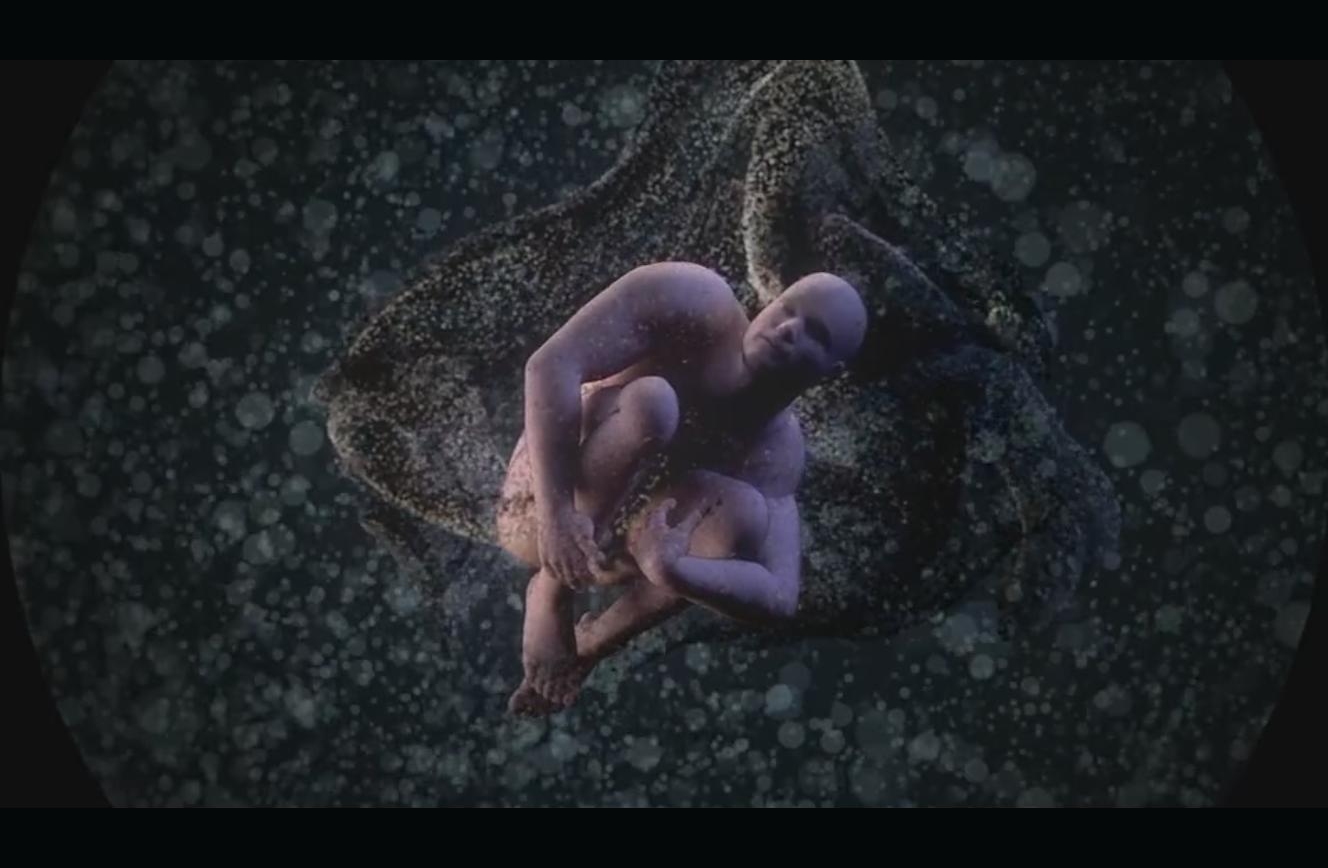
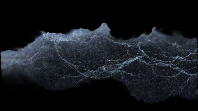
Stochastic shadowing in action, on something that is definately not an artistic interpretation of a sperm cell.
But there’s a twist: in order to improve the quality, cope with hash collisions and reduce aliasing, we perform a temporal reprojection step. When writing the shadow map each frame a random sub-pixel offset is applied to each particle which varies every frame; this means we get a different set of collisions, so different particles become visible each frame. Then when sampling the shadow map we blend the result with the previous frame, so the results adjust smoothly over time. By combining these two things we get a very nice, soft, reasonably alias-free shadow solution which is also efficient to render. No sorting required. The final shadow value per particle is written into a buffer and used at particle render time.
I also experimented with the technique for the actual rendering of the particles to the main frame – rendering single points with Z test and blurring the buffer out, with some per-pixel sorting during the composite, to create softened particles but without the need for a full particle sort. Unfortunately it didn’t give us the visual fidelity we needed; we relied on the blending of particles, the variable sizes and the sprites used. Could be more applicable in a future project though.
536. Meshing (Marching Cubes)
I suppose it’s the obvious step, isn’t it. Democoders love metaballs. Being able to render particles as meshes using metaballs is something we’ve wanted to do for ages because it moves us towards the “liquid” look – the Realflow-style look. We’ve been here before: in Frameranger we rendered around 50,000 metaballs in realtime by generating a potential field, converting it into a signed distance field and raymarching it. Results were promising but not perfect: being able to generate an actual triangle mesh has some side benefits, like being able to post process the mesh and adjust it with tension – something we really wanted to do to get closer to that Realflow look I keep going on about.
Marching cubes gives two issues to solve: generating the potentials, and then triangulating them. We already worked out how to generate the potentials some time ago for Frameranger, although a bit of work was required to scale it up to 250,000 particles. The second part is more difficult: you need to generate an arbitrary amount of geometry data from that potential field with triangle and vertex counts that change every frame. Naturally, we could quite easily make an implementation which just generates the worst case: treat every cell in the volume as if it was contributing triangles, then write degenerates for the invalid ones. That actually works – but it’s prohibitive for large volumes. One cell can contribute up to 5 triangles, and with a 128^3 volume we’d be looking at 10 million triangles – which isn’t great. 256^3 volumes would effectively be impossible. What we need is a way to only process and send triangles for the cells that are active.
This is problematic because we can’t generate index or vertex buffers on the GPU, we can’t generate drawcalls on the GPU (so we can’t vary how many primitives are rendered on the GPU) and we can’t use the CPU – because the potential field is on the GPU and it’d be far too slow to get it back to CPU. And even if we could, the CPU probably isn’t up to the task of generating the geometry fast enough anyway. And even if it was, we’d have to send all the triangle data back to the GPU again. So we’re stuck with the GPU – and yet we don’t have a way to vary the number of cells we render triangles for.
It seems impossible. However, Gernot Ziegler came up with a nice solution a while ago: histopyramids. This is a way of performing stream compaction on the GPU: it takes a big sparse buffer, and moves all the filled elements to the start of the buffer. A bit like a sort, but much more efficient. This gives us exactly what we need: we generate the (sparse) potential grid and use histopyramid compaction to move all the filled elements to the start. Then we use an occlusion query to count the number of active cells and use the CPU to generate batches which give enough triangles for the count to generate. The actual vertices are generated using a pixel shader and vertex texture fetch is used to read them.
Result!
4. Bokeh Glows
I’ve had this effect on the back burner for a few years but finally got to actually finishing it up.. Bokeh is the term relating to the effect of circular or shaped highlights in a depth of field effect, caused by inaccuracies in the shape of the lens of a camera. Or something. They make DOF look really nice. I’ve tried before by using a really big circular kernel for a regular DOF effect with an HDR input and leaving it at that and it actually does work, but I wanted to see if I could get some shaped bokehs and really overblow it. So I tried something with point sprites.
bokeh, innit. turned up to max, of course.
The basic idea is to work out where on screen bokehs would happen, and render point sprites at those points. I did this using the following method:
– Bilinear downsample the screen (in several steps), storing the 2d position (UV) of the brightest point of the 4 values of the quad that were read to a render target.
– Use those 2d positions to read a blurred version of the original frame. Perform some thresholding to pick out the points which pass. Generate colour values for the points.
– Temporally smooth positions and colours using positions from last frame, apply some attack and decay.
– Render a load of point sprites using vertex texture fetch to read the positions and colours, rendering the sprites to the screen. (With some additional magic to make it look good.)
72. Post Process Antialiasing (MLAA)
This is the first demo since 2009 (Frameranger, in fact) that we’ve released which actually features polygons being rendered as polygons. Happily, time has moved on, and so has our renderer. One of the major bugbears I had with the deferred renderer is lack of antialiasing – but fortunately a whole bunch of post process antialiasing techniques got invented in the last couple of years. MLAA is the technique du jour, and we use an implementation in our renderer. It’s great.
We do two little twists in our version to make it cool: firstly we use a lot of stencil optimisation so only the active edges get the big-ass shader applied to do the actual MLAA (or in fact get any of the process after the edge detect applied). And secondly.. there’s an ugly problem with MLAA in that it actually cocks up quite badly in a certain case. The technique relies on checking for horizontal or vertical edges. But where you have a pixel which is both a horizontal and vertical edge, it messes it up. Which breaks about 1/4 of the diagonal edges you have to deal with, so its pretty noticable. Our oh so clever technique for fixing that is.. do the MLAA twice. 🙂 The second time we flip the whole image in x and y, then MLAA it and flip it back. Genius huh? .. no? Well, it makes the polygonal scenes look good, and fortunately the stenciled version is so fast the extra hit isnt really noticable.
42. Stereoscopic 3D
We really wanted to do something with 3D for a while, but sadly we dont have any true 3D hardware (*cough* donations please *cough*). We decided quite early on that we were going to go for a pretty much black & white look – so it would actually be feasible to use the good old red / cyan anaglyph method. 3D isn’t as easy as just turning it on, though. It takes some effort to make it work well, give a good effect and not strain your eyes. We tuned it quite carefully and the setup of the scenes really helps – the first scene is slow and quite static so it lets your eyes adjust, the camera movements are quite smooth and in a single direction so they’re easy to track, and so on and so on.
Do watch the demo in 3D, it’s really made for it. We’re going to make a proper HD 3D video with left & right splits soon for those with real 3d setups.
End
I guess what’s interesting for me about this demo is that it was so much easier to make than many we’ve done. It just kind of came together; we started early enough, we got the music at the start, we didn’t have any major problems, nobody disappeared or dropped out, everything showed up on time, we didn’t completely overstretch ourselves and come up with some ideas that couldn’t be done, and we had time at the end to go over it and tweak and polish things, and we’re really happy with how it turned out. It’s like the way it’s supposed to go but never does. It doesn’t work for everyone (not very bombastic, you see) but it seems the people who got it really got it and like it, which is what matters. Maybe we’ve actually cracked it.. or maybe next time’ll be a royal screwup. Have to wait and see..
An amusing realisation hit me the other day. We’ve unintentionally managed to make a demo which is entirely full of sexual references. There’s a load of massive sperm cells; there’ what looks like a female gender symbol, made up of little sperm cells; there’s a load of sperm falling down and colliding off things; and then there’s a big river of .. well, it’s not much of a stretch in context to call that fluid “spunk”, is it? It only dawned on me after Dixan commented that it was “finally a good demo about semen” on pouet, and I started thinking about it.
To all the gamedev people who were savvy enough to get their company to pay for their plane ticket: come see me at GDC!
I’ll be introducing the new version of PhyreEngine – 3.0 – to the world. It has tools and everything. I’ll also be talking about the new rendering work we’ve done on PS3 lately. That includes:
-a particle system on SPU (which took a lot of ideas from the one ive presented on this blog which ran on GPU. but now on SPU.)
-a new take on MLAA on PS3
-deferred lighting on SPU and our rendering engine in general.
And then I get to talk about NGP. If you’re thinking of (or are currently) developing for the device, you might be interested in knowing what you can do on it graphics-wise and how it went adding NGP support for our engine. This I shall attempt to impart.
Plus, I’ll be giving out a free NGP devkit to the first 10 people through the door!* So come along! Thursday March 3rd, 3:00- 4:00, Room 302, South Hall.
(This is late. Really really late. Sorry. I’ve been busy! Honest.)
It’s become traditional for us to do something for Assembly (in Helsinki, Finland, 5-8 aug 2010). This year we wanted to do a demo that continued from Agenda with the particle theme, but took things further – we felt like we barely scratched the surface of what was possible. And we actually started quite early, almost three months before. The core plan and direction was laid down and we organised the soundtrack. We wanted to try and really plan something out and make something big.
100% particles
Unfortunately when man makes plans.. well, it completely didn’t work out. The soundtrack didn’t come out as we hoped, the demo plot was far too bound to the soundtrack and the visuals were far too bound to the plot – we were at the mercy of it. Every scene was required, every part needed for it to make sense. We realised the whole thing wasn’t going to happen. So we started again. We hunted around for possible tracks and in the end Hunz came to the rescue – he let us use his beautiful track “All Falls Down” and also remixed it for us to fit the direction on a very short timescale.
So about that direction – well, the original plan for the demo was this sort of time-shifted end-of-the-world meet your maker theme where a city gets destroyed by some sort of holocaust, but then a phoenix rises from its ashes. It was going to be great! Trust me. Well, happily the new soundtrack – with strong vocals leading the way – actually did support this theme, but we were able to do something more loose than we had originally planned – disaster-related scenes, but less of a central plot to be reliant on.
Naturally the engine had matured a bit since Agenda, and we now benefitted from overall better performance, as well as a number of new features and effects; in particular lines / hair, displacement mapping of particles and collisions with distance fields. There were also a few effects I made specifically for the demo: fire using fluid solvers, raytraced spheres and a tidal wave thing. I’ll go through some of those in turn.
Hair
A natural step when you’ve got a particle system is to try linking the particles together with lines so you get something like hair, and that’s how this started out. Then you’ve got two immediate issues to overcome: how to get the right particles linked together so it isn’t a jumbled mess; and how to make them move in a way that appears connected. Fortunately if you solve the latter you’re a long way to fixing the former.
Firstly, we assume that particles next to each other in the texture are part of the same line, up until some line length is reached. For simplicity’s sake all the lines contain the same number of particles, and that number is a power of two so a number of lines fit neatly into the particle texture. Lines are arranged solely in the X direction of the particle texture and can’t spread onto multiple rows: i.e. the maximum line length allowed is the width of the particle texture. With this arrangement you’ve got a pretty easy way of finding the particles that make up one line, of finding the next and previous particles in the line and so on. For example, in a 1024×1024 particle texture and a line length of 256, I have 4 lines per row – 4096 lines in total.
Connected movement is achieved by using a spring solver. Particles attempt to maintain a certain distance from their connected neighbours in a line by pushing and pulling towards them; several iterations of that are performed per update. So it’s simply a case of looking at the next and previous particles in the line and moving the particle towards or away from its neighbours as appropriate. End points can be anchored if we want.
Ah, but why do the previous and next particles actually make sense as line neighbours in the first place? Can’t they be anywhere in space? No, because I have a special emitter that emits particles in a suitable way – i.e. as lines in the first place. This can be done using a random direction, or using normals from a mesh, or to fill a mesh, or along contours of a distance field. If they start off in a good shape, and there’s a spring solver on them to keep them in a good shape, they stay in a good shape. Easy.
For rendering we have a couple of options: line primitives or camera-facing quad strips. Quads have the advantage of having actual thickness, but they’re slower to render and have to be at least a minimum thickness or they get culled by the hardware. We tessellate at render time using catmull rom splines so lines can be smoother – that’s just done in the vertex shader. We use opacity shadow maps just like the particles use – so the lines are self shadowed nicely.
The shading had quite a lot of faking involved too, actually. I used a blend between a few colours; a dark tone which is used as an “occluded” colour near the root, and a lighter “unoccluded” tone; then a couple of tones to randomly pick between for each strand of hair.
*Unreleased material alert!* The hair effect when used on a horse, a while ago
Naturally as with all these particle things, the issue isn’t about numbers, it’s about control – and that was the trick: emitting to fill a mesh (a match stick in this case), getting all blown about and then reforming into that mesh again. It turned out the curl noise affector worked great on lines because it has spatial continuity – it made it look like hair underwater, which is exactly what we wanted.
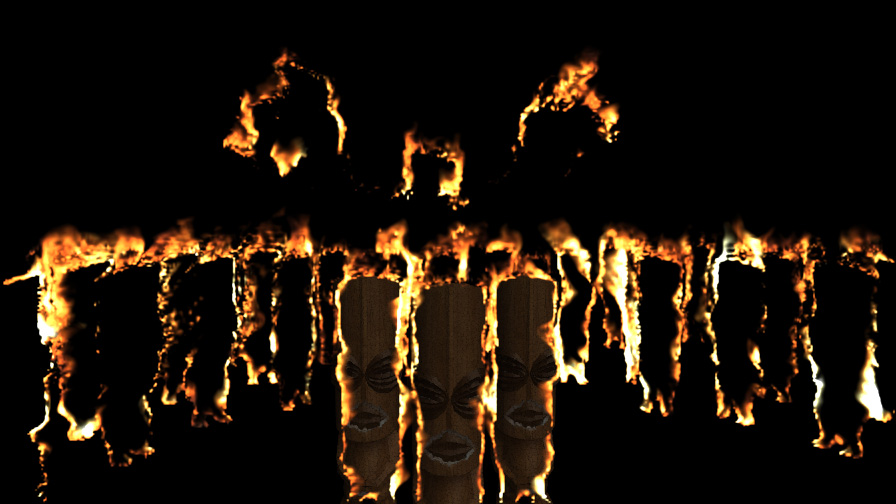
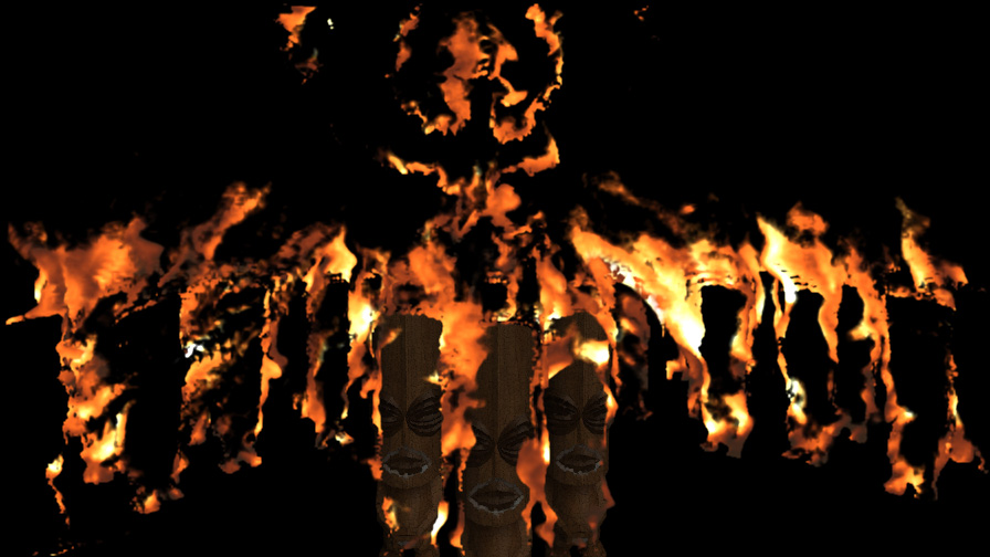
Fire
I spent some time looking into how to do a good fire effect with the help of some Siggraph papers. Fire is quite hard to do properly – you have to capture the large-scale and small-scale movements. The really good way to do fire is to use a massive 3D fluid solver which is big enough to capture the small-scale details – but that’s completely prohibitive in terms of memory and performance. So there’s an approximation. The basic theory is, you use a small number of screen-aligned 2D slices each running their own separate 2D fluid solver; and you blend the input velocity and density across the slices so they all have pretty similar source data, which means they all move in a way that makes sense across the slices. Then you add some procedural fluid flow (read: curl noise) on top to add detail.
The way I started was to follow the paper and use particles for inputs. You render them as particles extruded into quads to capture the motion, rendering both density & temperature and velocity into the slices as MRTs; then you apply 2D fluid solvers to the slices, apply some procedural motions and render the slices view aligned with some shader to generate colour from temperature. Well, it turned out to be a total bitch. It appeared the paper left out a few critical details, and it didn’t work out quite the way I hoped. The biggest problem was one of scale – getting a fire that would work for a big volume of it – like the heads of some tikis – was very different to one that worked for a small one like the burning head of a match. Also we couldnt get quite as many slices as we wanted because it was just too heavy with large, high resolution fluid simulations, even in 2D. The particles also didn’t give a clean and smooth enough result, even when extruded into quads.
In the end we ditched particles as inputs totally and used meshes instead. Well, GBuffers anyway. I rendered the meshes to GBuffers and blended those into the fire buffers, weighted by depth from slice and generating velocities using perlin noise and the screen space normals. This gave a much cleaner result which was more controllable and a massive amount faster. Still a total bitch to get the scales working well for different fires, though.
Evolution of the fire effect
See, it got better
And then there was the rendering. You would think it’d be easy to map a floating point temperature value into good looking colours, but it wasn’t. I also had to blend them across the slices and with other scene elements, and there just didn’t seem to be a mode that made it look good. It took an age of tweaking and I never was satisfied with it.
In the end we got.. something. I wasn’t totally happy with the effect but it did add something to the demo that wasn’t particles. It looked pretty good when applied to that fucking phoenix at the end though.
Raytraced spheres
Problem: render a reasonably large number (lets say 100s) of moving spheres that can overlap in screen space, and are all refractive, with a reasonable degree of accuracy. Solution? Lets see.. they need to refract the background which is easily achieved through render to texture; that alone could be achieved with a simple rasterisation-based approach. But they also need to refract each other given that they could overlap a lot – and that overlapping makes rasterisation inappropriate, and a raytracing solution would be better. Oh, and we also need it to not eat too much frame time given that it’s a small part of a much larger scene, so that – combined with the large number of spheres – prohibits a simple brute force approach of checking the ray against each sphere per pixel and then again for the refractions.
Raytraced spheres turned into particles, early in development. This effect was a right pain
What I needed was a way of reducing the problem down to a smaller set of spheres per pixel which are likely to affect the ray at that pixel. One way would be to build a 3D spatial database for the spheres and use that to trace more efficiently, but that isn’t all that pixel shader friendly – or easy to update per frame. So I cut a few corners and went for a 2D approach. The idea was, at a low resolution I worked out which spheres overlapped each pixel and stored those spheres in render targets; then at a high resolution I only consider the spheres in those render targets to trace through, rather than all of them. In order to cope with refractions I had to be a bit generous on the overlap test, but it worked well. The low resolution classification step was a long shader that looped through the large number of spheres – sorted front to back and roughly pre-classified on CPU to only check those vaguely near the pixel – and gathered the first 4 that overlapped, writing them to MRTs. The high resolution tracing shader loaded the 4 spheres from the render targets and checked them for ray intersections, then traced the ray through for refractions, finally getting an exit direction to look up the back buffer. 4 spheres was usually enough overlap to get believeable refractions – and hey, we were going to turn it all into particles anyway, so there was room for error.. wait, what was that about overkill?
I’ve used this approach before to render large numbers of metaballs (1000s) too; the problem is that with a lot of balls you start to need a lot of overlapped spheres per pixel, and you simply can’t cache enough, so it breaks down. To do 1000s of metaballs you need a different approach, but that’s something for another post..
Particle fun
One of the main scenes in the demo involves a street of buildings which gets blown up, building at a time, into particle explosions. That got.. pretty heavy. Each building was built of 1m particles, so we ended up pushing 10m particles per frame through the render. Ow. That was just not going to fly as regular particles where we maxed out any reasonable GPU at 2m – and blew all kinds of memory limits with more than that – so we had to do some things to cut it down.
New PC shadebob record
The first idea was “static particles”. The idea was, don’t do all the simulation and sorting the particles go through; just use the position and colour textures that were pregenerated for emission from a mesh, and pass them straight to the particle renderer. The particles could be pre-sorted in that texture for a rough camera direction so it looked alright. This obviously slices the amount of work done per frame a lot. The particles would be static though, but we could use displacement mapping effects (see later) to add some movement. We could also fake them fading in and out for lifetime cycles.
This trick bought us a lot of the time back; we could actually render the scene with this and get some sort of sensible framerate. But we didn’t want a static scene, we wanted to explode the buildings. So I devised a scheme of smoke and mirrors, whereby a building is static particles until it explodes, and then switches seamlessly to a proper particle system. Buut, you cant very well keep them all as particle systems after explode because it wastes loads of VRAM, which we’re already pushing too hard; so I wait until the explosion gets almost static and then switch them to an imposter by rendering them to a texture.
Displacement Mapping
Displacement mapping was used to add a per-frame offset to particle positions. This is done at render time only; well, not actually in the vertex shader, but as a pre-pass just before the render which processes the position buffer. It’s means it’s a temporary operation – it doesn’t have to persist to the next frame so it’s not part of the simulation, so the results don’t get stored and eat memory. So it works on static particles like on the street scene, which is ideal because we needed to add some movement there.
I added a bunch of operators – audio-based FFT modifiers, perlin noise movement modifiers, and things using images. We used it for some pulsing audio effects and a few other bits and pieces. Simple but oh, so effective.
Depth of field
Jani came up with this and it worked out a total treat. The idea is that we had so many particles that we could achieve a depth of field look just by randomising the positions a bit at render time (in vertex shader), where the randomness is controlled by the distance from focus. It took a fair few goes for him to explain it to me in a way that I understood, but once we got there I added it and it totally worked – it looked great. We could use it for focus pulls, “blurring out” shots and so on.
Particle randomisation for depth of field
Distance fields
The subject of collisions with particles against meshes had come up before. Like that of real particle fluids – i.e. SPH – or rigid bodies or meshing, it usually get met with “in realtime? fuck off” or “yea.. I bet in 5 years we’ll be doing that” or “I’ll get to it when I’m done adding the radiosity solver” or some other smartass coder vs artist remark. Like what we used to say about shadows in the 90s. Of course, those arguments always end up evaporating because it actually gets done in the end when someone comes up with a practical, simple, workable way of doing it. And so it is here. All the hype about distance fields made me get around to writing a proper mesh to signed distance field conversion routine for some effect or other, and I realised it would make perfect sense to use for particle collisions. With meshes.
It’s a pretty simple routine; get the particle position in the space of the distance field, see if it’s inside, work back to find the 0 contour and the field normal at the hit point and then do something. Like move the particle and set some bounce velocity. So I did it and we used it with the tidal wave scenes, and it was great! Particles colliding with logos, with 3d scenes, and so on.
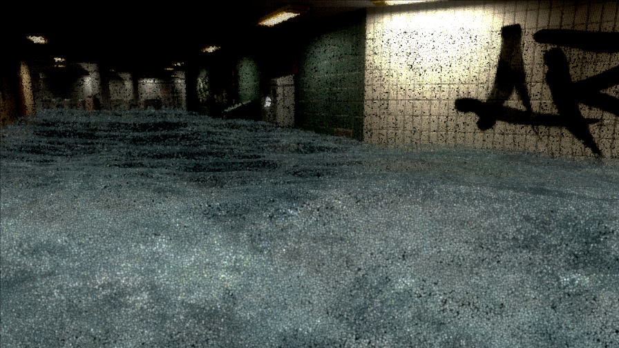
Well, it would have been great if the routine had worked. It didn’t; the mesh to distance field conversion was broken, so parts of the field were all wrong and it produced all kind of funny results. We managed to fudge the effect enough to get through the demo but it wasn’t until months later that I realised the mistakes and made something that really worked properly. In the demo it works in a few places but it’s not quite what it should have been.. so you get a few splashes off the logo and some collisions with what basically ended up as boxes in the subway scene.
The good news is I fixed it since, and it’s brilliant. So many applications for it; although the real challenge is in getting an accurate signed distance field of an arbitrary complex mesh efficiently in the first place, and that was what took so long to solve. It probably deserves a whole article on it’s own so let’s leave it there.
Water
I don’t know how this came about, but someone – might have been me actually – had the idea of using an ocean water effect and making the particles follow it. That water routine is so old. I’ve had it working since about 2003 and never actually used it in a demo, although it was planned for a couple and didn’t make it. It’s the implementation of Tessendorf’s FFT-based ocean water simulation, and it gives you a nice realistic ocean water heightfield which people usually use for meshes. I remember at the time I wrote it it worked fast on something like 32×32 or 64×64 grids on a PC CPU (due to the inverse 2D FFT you need to do), which wasn’t all that good looking. Since then Caspar did one on the PS3 running on SPU which ran at 256×256 if I remember right; fortunately PC CPUs caught up and now I can run it at a decent resolution pretty comfortably. If you want to know how the ocean routines work, google Tessendorf FFT ocean water and you’ll no doubt be presented with a load of material.
Original version of the water effect
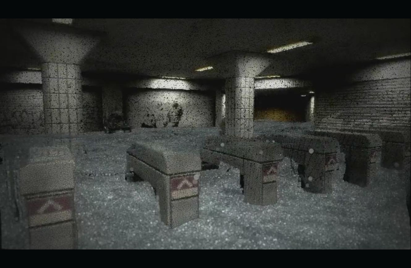
The water in the subway scene, later
That was the first step; but then we started messing with it. We had a subway scene where we wanted to fill it with water and make it look like a wave was crashing through it. In an ideal (fantasy) world that would be done with proper fluid dynamics; I thought it’d be better (i.e. achieveable) if we faked it by taking the ocean effect and applying some magical space modifier to it to warp it into the shape of a wave. Simple.. a wave curl is a bit like some warped bell curve shifted and curled around by a twist / vortex equation. Right? Except somehow I was attempting to do this really late at night not all that long before the deadline, and I just couldn’t get it for ages and ages. GCSE maths is hard.
The subway scene
Post Processing
I have to quickly mention the post processing effects – well, effect – that we used to make the screen all break up and look like a broken video recording. A lot of people moaned about it, some liked it. Personally I love it. It’s a combination of a load of different small things which go together to make something cool. We mix between a load of distortions using sinewaves and noise – some on scanlines, some on blocks; stretching, offseting and flipping the screen; and then this frame-holding effect where we keep a history of a few frames and randomly hold them or jump between them for a little while. There’s something really satisfying about taking a scene you’ve spent ages lovingly crafting, and then messing it up on purpose.
So there it is – we tried to make plans, it didn’t work out, and we made something much quicker instead. I’m really glad I got to work with Hunz, and I’m happy with some of the routines that were put together pretty fast. Demo compos, like war, can be the source of great innovation and technical advancement – if things have to get done, they get done. Yep, demo compos are a lot like war actually. Except you can watch them with a few beers in the grandstand of a hockey arena, not on CNN.
I happened to do a seminar at Assembly which is here – if you want to watch 50 minutes of me discussing how we made our recent demos and at the same time being a cocky little shit. Go on, you know you want to.
Coming soon: all the new things we’ve been doing between when the content of this blog post was actually fresh and relevant, and now..
Look, sorry – I’ve not updated this blog in months and I feel a bit bad about it. It’s not because I’ve given up on the whole thing and become a hermit living on herring in the uninhabited part of the scottish isles – oh no. It’s the opposite – I’ve been so busy actually making shit that I havent had time to finish that big writeup of Ceasefire that’s been sitting in the outbox for months, let alone talk about all the new things we’ve got going on that you’ll see soon enough. They make the old stuff look a bit silly.
But anyway. Just wanted to mention: we got some nominations for the Scene.org Awards 2010. Ceasefire got nods for best demo and best soundtrack (for Hunz – well deserved!), and Agenda Circling Forth scored a record 7 nominations: best demo, graphics, effects, direction, original concept, technical achievement and public’s choice. Our c64 superstars also got a nomination for best demo on an oldschool platform for We Are New.
You can actually vote in the public choice category (for us) right now if you feel like it.
Filed under: Uncategorized — directtovideo @ 8:32 am
Just wanted to mention – Agenda Circling Forth got shown in the Live Realtime Demos show at Siggraph 2010!
This show was strictly speaking for interactive pieces only, and ours was a realtime non-interactive demo. So I did some work to make it interactive via the use of a webcam – basically you can wave your hands around in front of the camera and it uses optical flow to calculate a motion buffer, which is used to manipulate the velocities of the particles, the fluid effects and the intensity of some of the post processing. It worked out quite nicely actually. I might have to make an exe available at some point..
I wasn’t able to attend in person so my friend Steve McAuley kindly presented it at the show. Unfortunately there were some technical difficulties at the show and when they attached a webcam to the PC it made it really unstable, so they ended up showing the non-interactive version. Still, the work on interactivity isn’t wasted – I’m sure it’ll be useful for other projects in future.
Many thanks to the organisers and to Steve for doing the business over there. Hopefully we’ll be able to do this again in future.