real time ray tracing part 2.

Here’s the science bit. Concentrate..

In the last post I gave an overview of my journey through realtime raytracing and how I ended up with a performant technique that worked in a production setting (well, a demo) and was efficient and useful. Now I’m going go into some more technical details about the approaches I tried and ended up using.

There’s a massive amount of research in raytracing, realtime raytracing, GPU raytracing and so on. Very little of that research ended up with the conclusions I did – discarding the kind of spatial database that’s considered “the way” (i.e. bounding volume hierarchies) and instead using something pretty basic and probably rather inefficient (regular grids / brick maps). I feel that conclusion needs some explanation, so here goes.

I am not dealing with the “general case” problem that ray tracers usually try and solve. Firstly, my solution was always designed as a hybrid with rasterisation. If a problem can be solved efficiently by rasterisation I don’t need to solve it with ray tracing unless it’s proved that it would work out much better that way. That means I don’t care about ray tracing geometry from the point of view of a pin hole camera: I can just rasterise it instead and render out GBuffers. The only rays I care about are secondary – shadows, occlusion, reflections, refractions – which are much harder to deal with via rasterisation. Secondly I’m able to limit my use case. I don’t need to deal with enormous 10 million poly scenes, patches, heavy instancing and so on. My target is more along the lines of a scene consisting of 50-100,000 triangles – although 5 Faces topped that by some margin in places – and a reasonably enclosed (but not tiny .. see the city in 5 Faces) area. Thirdly I care about data structure generation time. A lot. I have a real time fully dynamic scene which will change every frame, so the data structure needs to be refreshed every frame to keep up. It doesn’t matter if I can trace it in real time if I can’t keep the structure up to date. Forthly I have very limited scope for temporal refinement – I want a dynamic camera and dynamic objects, so stuff can’t just be left to refine for a second or two and keep up. And fifth(ly), I’m willing to sacrifice accuracy & quality for speed, and I’m mainly interested in high value / lower cost effects like reflections rather than a perfect accurate unbiased path trace. So this all forms a slightly different picture to what most ray tracers are aiming for.

Conventional wisdom says a BVH or kD-Tree will be the most efficient data structure for real time ray tracing – and wise men have said that BVH works best for GPU tracing. But let’s take a look at BVH in my scenario:
– BVH is slow to build, at least to build well, and building on GPU is still an open area of research.
– BVH is great at quickly rejecting rays that start at the camera and miss everything. However, I care about secondary rays cast off GBuffers: essentially all my rays start on the surface of a mesh, i.e. at the leaf node of a BVH. I’d need to walk down the BVH all the way to the leaf just to find the cell the ray starts in – let alone where it ends up.
– BVH traversal is not that kind to the current architecture of GPU shaders. You can either implement the traversal using a stack – in which case you need a bunch of groupshared memory in the shader, which hammers occupancy. Using groupshared, beyond a very low limit, is bad news mmkay? All that 64k of memory is shared between everything you have in flight at once. The more you use, the less in flight. If you’re using a load of groupshared to optimise something you better be smart. Smart enough to beat the GPU’s ability to keep a lot of dumb stuff in flight and switch between it. Fortunately you can implement BVH traversal using a branching linked list instead (pass / fail links) and it becomes a stackless BVH, which works without groupshared.
But then you hit the other issue: thread divergence. This is a general problem with SIMD ray tracing on CPU and GPU: if rays executed inside one SIMD take different paths through the structure, their execution diverges. One thread can finish while others continue, and you waste resources. Or, one bad ugly ray ends up taking a very long time and the rest of the threads are idle. Or, you have branches in your code to handle different tree paths, and your threads inside a single wavefront end up hitting different branches continually – i.e. you pay the total cost for all of it. Dynamic branches, conditional loops and so on can seriously hurt efficiency for that reason.
– BVH makes it harder to modify / bend rays in flight. You can’t just keep going where you were in your tree traversal if you modify a ray – you need to go back up to the root to be accurate. Multiple bounces of reflections would mean making new rays.

All this adds up to BVH not being all that good in my scenario.

So, what about a really really dumb solution: storing triangle lists in cells in a regular 3D grid? This is generally considered a terrible structure because:
– You can’t skip free space – you have to step over every cell along the ray to see what it contains; rays take ages to work out they’ve hit nothing. Rays that hit nothing are actually worse than rays that do hit, because they can’t early out.
– You need a high granularity of cells or you end up with too many triangles in each cell to be efficient, but then you end up making the first problem a lot worse (and needing lots of memory etc).

However, it has some clear advantages in my case:
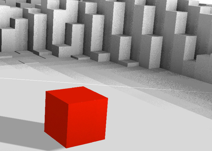
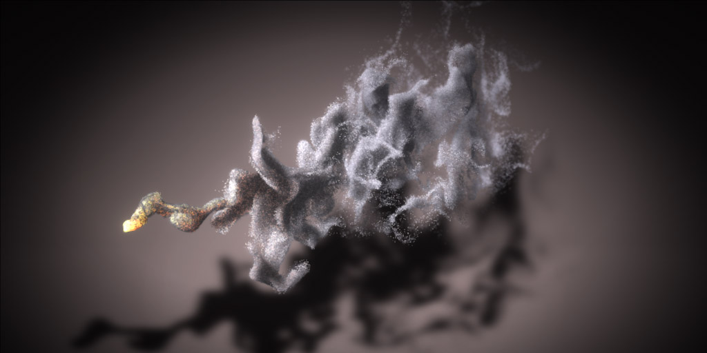
– Ray marching voxels on a GPU is fast. I know because I’ve done it many times before, e.g. for volumetric rendering of smoke. If the voxel field is quite low res – say, 64x64x64 or 128x128x128 – I can march all the way through it in just a few milliseconds.
– I read up on the DDA algorithm so I know how to ray march through the grid properly, i.e. visit every cell along the ray exactly once 🙂
– I can build them really really fast, even with lots of triangles to deal with. To put a triangle mesh into a voxel grid all I have to do is render the mesh with a geometry shader, pass the triangle to each 2D slice it intersects, then use a UAV containing a linked list per cell to push out the triangle index on to the list for each intersected cell.
– If the scene isn’t too high poly and spread out kindly, I don’t have too many triangles per cell so it intersects fast.
– There’s hardly any branches or divergence in the shader except when choosing to check triangles or not. All I’m doing is stepping to next cell, checking contents, tracing triangles if they exist, stepping to next cell. If the ray exits the grid or hits, the thread goes idle. There’s no groupshared memory requirement and low register usage, so lots of wavefronts can be in flight to switch between and eat up cycles when I’m waiting for memory accesses and so on.
– It’s easy to bounce a ray mid-loop. I can just change direction, change DDA coefficients and keep stepping. Indeed it’s an advantage – a ray that bounces 10 times in quick succession can follow more or less the same code path and execution time as a ray that misses and takes a long time to exit. They still both just step, visit cells and intersect triangles; it’s just that one ray hits and bounces too.

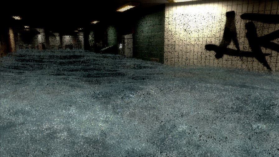
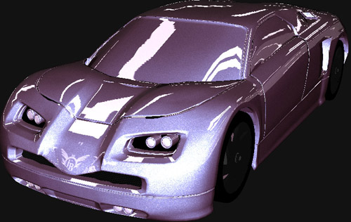
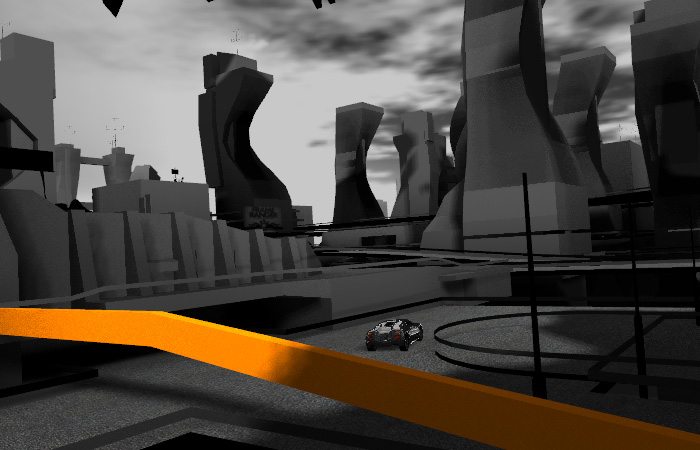
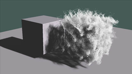
Gratuitous screenshot from 5 Faces

So this super simple, very poor data structure is actually not all that terrible after all. But it still has some major failings. It’s basically hard limited on scene complexity. If I have too large a scene with too many triangles, the grid will either have too many triangles per cell in the areas that are filled, or I’ll have to make the grid too high res. And that burns memory and makes the voxel marching time longer even when nothing is hit. Step in the sparse voxel octree (SVO) and the brick map.

Sparse voxel octrees solve the problem of free space management by a) storing a multi-level octree not a flat grid, and b) only storing child cells when the parent cells are filled. This works out being very space-efficient. However the traversal is quite slow; the shader has to traverse a tree to find any leaf node in the structure, so you end up with a problem not completely unlike BVH tracing. You either traverse the whole structure at every step along the ray, which is slow; or use a stack, which is also slow and makes it hard to e.g. bend the ray in flight. Brick maps however just have two discrete levels: a low level voxel grid, and a high level sparse brick map.

In practice this works out as a complete voxel grid (volume texture) at say 64x64x64 resolution, where each cell contains a uint index. The index either indicates the cell is empty, or it points into a buffer containing the brick data. The brick data is a structured buffer (or volume texture) split into say 8x8x8 cell bricks. The bricks contain uints pointing at triangle linked lists containing the list of triangles in each cell. When traversing this structure you step along the low res voxel grid exactly as for a regular voxel grid; when you encounter a filled cell you read the brick, and step along that instead until you hit a cell with triangles in, and then trace those.

The key advantage over an SVO is that there’s only two levels, so the traversal from the top down to the leaf can be hard coded: you read the low level cell at your point in space, see if it contains a brick, look up the brick and read the brick cell at your point in space. You don’t need to branch into a different block of code when tracing inside a brick either – you just change the distance you step along the ray, and always read the low level cell at every iteration. This makes the shader really simple and with very little divergence.

Brick map generation in 2D

Building a brick map works in 3 steps and can be done sparsely, top down:
– Render the geometry to the low res voxel grid. Just mark which cells are filled;
– Run over the whole grid in a post process and allocate bricks to filled low res cells. Store indices in the low res grid in a volume texture
– Render the geometry as if rendering to a high res grid (low res size * brick size); when filling in the grid, first read the low res grid, find the brick, then find the location in the brick and fill in the cell. Use a triangle linked list per cell again. Make sure to update the linked list atomically. 🙂

The voxel filling is done with a geometry shader and pixel shader in my case – it balances workload nicely using the rasteriser, which is quite difficult to do using compute because you have to load balance yourself. I preallocate a brick buffer based on how much of the grid I expect to be filled. In my case I guess at around 10-20%. I usually go for a 64x64x64 low res map and 4x4x4 bricks for an effective resolution of 256x256x256. This is because it worked out as a good balance overall for the scenes; some would have been better at different resolutions, but if I had to manage different allocation sizes I ran into a few little VRAM problems – i.e. running out. The high resolution is important: it means I don’t have too many tris per cell. Typically it took around 2-10 ms to build the brick map per frame for the scenes in 5 Faces – depending on tri count, tris per cell (i.e. contention), tri size etc.

One other thing I should mention: where do the triangles come from? In my scenes the triangles move, but they vary in count per frame too, and can be generated on GPU – e.g. marching cubes – or can be instanced and driven by GPU simulations (e.g. cubes moved around on GPU as fluids). I have a first pass which runs through everything in the scene and “captures” its triangles into a big structured buffer. This works in my ubershader setup and handles skins, deformers, instancing, generated geometry etc. This structured buffer is what is used to generate the brick maps in one single draw call. Naturally you could split it up if you had static and dynamic parts, but in my case the time to generate that buffer was well under 1ms each frame (usually more like 0.3ms).

Key brick map advantages:
– Simple and fast to build, much like a regular voxel grid
– Much more memory-efficient than a regular voxel grid for high resolution grids
– Skips (some) free space
– Efficient, simple shader with no complex tree traversal necessary, and relatively little divergence
– You can find the exact leaf cell any point in space is in in 2 steps – useful for secondary rays
– It’s quite possible to mix dynamic and static content – prebake some of the brick map, update or append dynamic parts
– You can generate the brick map in camera space, world space, a moving grid – doesn’t really matter
– You can easily bend or bounce the ray in flight just like you could with a regular voxel grid. Very important for multi-bounce reflections and refractions. I can limit the shader execution loop by number of cells marched not by number of bounces – so a ray with a lot of quick local bounces can take as long as a ray that doesn’t hit anything and exits.

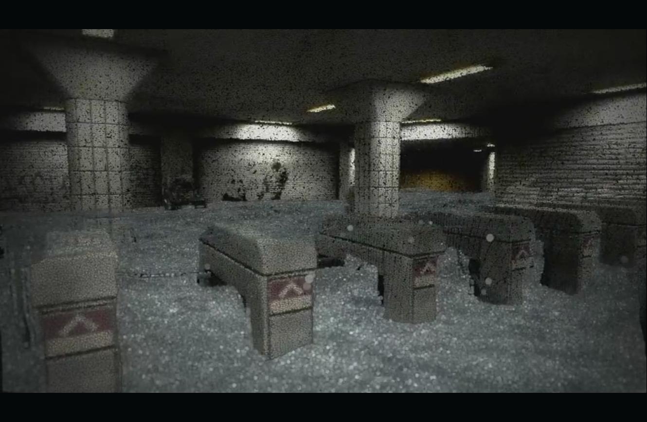
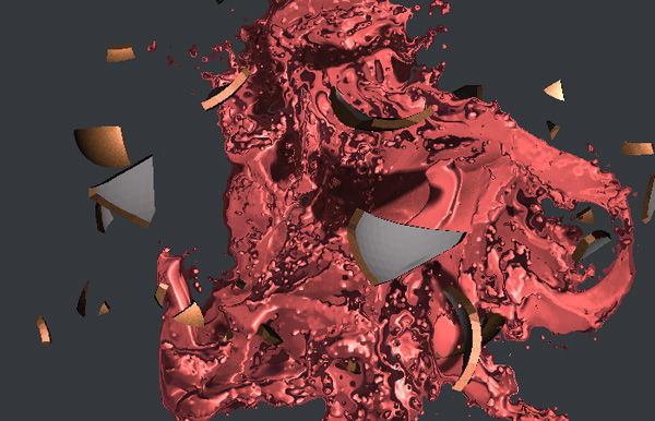
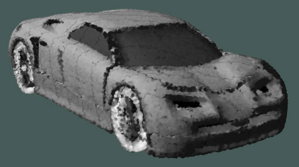
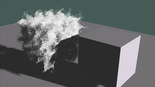
Gratuitous screenshot from 5 Faces

In conclusion: brick maps gave me a fast, efficient way of managing triangles for my real time raytracer which has a very particular use case and set of limitations. I don’t want to handle camera rays, only secondary rays – i.e. all of my rays start already on a surface. I don’t need to handle millions of triangles. I do need to build the structure very quickly and have it completely dynamic and solid. I want to be able to bounce rays. From a shader coding point of view, I want as little divergence as possible and some control over total execution time of a thread.

I don’t see it taking over as the structure used in Octane or Optix any time soon, but for me it definitely worked out.

real time ray tracing.

It’s practically a tradition.

New hardware generation, new feature set. Ask the age old question: “is real time ray tracing practical yet?”. No, no it’s not is the answer that comes back every time.

But when I moved to Directx 11 sometime in the second half of 2011 I had the feeling that maybe this time it’d be different and the tide was changing. Ray tracing on GPUs in various forms has become popular and even efficient – be it in terms of signed distance field tracing in demos, sparse voxel octrees in game engines, nice looking WebGL path tracers, or actual proper in-viewport production rendering tracers like Brigade / Octane . So I had to try it.

My experience of ray tracing had been quite limited up til then. I had used signed distance field tracing in a 64k, some primitive intersection checking and metaball tracing for effects, and a simple octree-based voxel tracer, but never written a proper ray tracer to handle big polygonal scenes with a spatial database. So I started from the ground up. It didn’t really help that my experience of DX11 was quite limited too at the time, so the learning curve was steep. My initial goal was to render real time sub surface scattering for a certain particular degenerate case – something that could only be achieved effectively by path tracing – and using polygonal meshes with thin features that could not be represented effectively by distance fields or voxels – they needed triangles. I had a secondary goal too; we are increasingly using the demo tools to render things for offline – i.e. videos – and we wanted to be able to achieve much better render quality in this case, with the kind of lighting and rendering you’d get from using a 3d modelling package. We could do a lot with post processing and antialiasing quality but the lighting was hard limited – we didn’t have a secondary illumination method that worked with everything and gave the quality needed. Being able to raytrace the triangle scenes we were rendering would make this possible – we could then apply all kinds of global illumination techniques to the render. Some of those scenes were generated on GPU so this added an immediate requirement – the tracer should work entirely on GPU.

I started reading the research papers on GPU ray tracing. The major consideration for a triangle ray tracer is the data structure you use to store the triangles; a structure that allows rays to quickly traverse space and determine if, and what, they hit. Timo Aila and Samuli Laine in particular released a load of material on data structures for ray acceleration on GPUs, and they also released some source. This led into my first attempt: implementing a bounding volume hierarchy (BVH) structure. A BVH is a tree of (in thise case) axis aligned bounding boxes. The top level box encloses the entire scene, and at each step down the tree the current box is split in half at a position and axis determined by some heuristic. Then you put the triangles in each half depending on which one they sit inside, then generate two new boxes that actually enclose their triangles. Those boxes contain nodes and you recurse again. BVH building was a mystery to me until I read their stuff and figured out that it’s not actually all that complicated. It’s not all that fast either, though. The algorithm is quite heavyweight so a GPU implementation didn’t look trivial – it had to run on CPU as a precalc and it took its time. That pretty much eliminated the ability to use dynamic scenes. The actual tracer for the BVH was pretty straightforward to implement in pixel or compute shader.

Finally for the first time I could actually ray trace a polygon mesh efficiently and accurately on GPU. This was a big breakthrough – suddenly a lot of things seemed possible. I tried stuff out just to see what could be done, how fast it would run etc. and I quickly came to an annoying conclusion – it wasn’t fast enough. I could trace a camera ray per pixel at the object at a decent resolution in a frame, but if it was meant to bounce or scatter and I tried to handle that it got way too slow. If I spread the work over multiple frames or allowed it seconds to run I could achieve some pretty nice results, though. The advantages of proper ambient occlusion, accurate sharp shadow intersections with no errors or artefacts, soft shadows from area lights and so on were obvious.

An early ambient occlusion ray tracing test

Unfortunately just being able to ray trace wasn’t enough. To make it useful I needed a lot of rays, and a lot of performance. I spent a month or so working on ways to at first speed up the techniques I was trying to do, then on ways to cache or reduce workload, then on ways to just totally cheat.

Eventually I had a solution where every face on every mesh was assigned a portion of a global lightmap, and all the bounce results were cached in a map per bounce index. The lightmaps were intentionally low resolution, meaning fewer rays, and I blurred it regularly to spread out and smooth results. The bounce map was also heavily temporally smoothed over frames. Then for the final ray I traced out at full resolution into the bounce map so I kept some sharpness. It worked..

.. But it wasn’t all that quick, either. It relied heavily on lots of temporal smoothing & reprojection, so if anything moved it took an age to update. However this wasn’t much of a problem because I was using a single BVH built on CPU – i.e. it was completely static. That wasn’t going to do.

At this point I underwent something of a reboot and changed direction completely. Instead of a structure that was quite efficient to trace but slow to build (and only buildable on CPU), I moved to a structure that was as simple to build as I could possibly think of: a voxel grid, where each cell contains a list of triangles that overlap it. Building it was trivial: you can pretty much just render the mesh into the grid and use a UAV to write out the triangle indices of triangles that intersect the voxels they overlapped. Tracing it was trivial too – just ray march the voxels, and if the voxel contains triangles then trace the triangles in it. Naturally this was much less efficient to trace than BVH – you could march over multiple cells that contain the same triangles and had to test them again, and you can’t skip free space at all, you have to trace every voxel. But it meant one important thing: I could ray trace dynamic scenes. It actually worked.

At this point we started work on an ill fated demo for Revision 2012 which pushed this stuff into actual production.

 

 
 
 
 
 
 
 
 

It was here we hit a problem. This stuff was, objectively speaking, pretty slow and not actually that good looking. It was noisy, and we needed loads of temporal smoothing and reprojection so it had to move really slowly to look decent. Clever though it probably was, it wasn’t actually achieving the kind of results that made it stand up well enough on its own to justify the simple scenes we were limited to being able to achieve with it. That’s a hard lesson to learn with effect coding: no matter how clever the technique, how cool the theory, if it looks like a low resolution baked light map but takes 50ms every frame to do then it’s probably not worth doing, and the audience – who naturally finds it a lot harder than the creator of the demo to know what’s going on technically – is never going to “get it” either. As a result production came to a halt and in the end the demo was dropped; we used the violinist and the soundtrack as the intro sequence for Spacecut (1st place at Assembly 2012) instead with an entirely different and much more traditional rendering path.

The work I did on ray tracing still proved useful – we got some new tech out of it, it taught me a lot about compute, DX11 and data structures, and we used the BVH routine for static particle collisions for some time afterwards. I also prototyped some other things like reflections with BVH tracing. And here my ray tracing journey comes to a close.

Ray tracing – unreleased Revision demo, 2012

Ray tracing – unreleased Revision demo, 2012

 
 
 
 
 
 
 
 
 
 
 
 

 
 
 
 
 
 
 
 
 
 
 
 

 
 
 
 
 
 
 
 
 
 
 
 

 
 
 
 
 
 
 
 
 
 
 
 

 
 
 
 
 
 
 
 
 
 
 
 
 
 

.. Until the end of 2012.

In the interim I had been working on a lot of techniques involving distance field meshing, fluid dynamics and particle systems, and also volume rendering techniques. Something that always came up was that the techniques typically involved discretising things onto a volume grid – or at least storing lists in a volume grid. The limitation was the resolution of the grid. Too low and it didn’t provide enough detail or had too much in each cell; too high and it ate too much memory and performance. This became a brick wall to making these techniques work.

One day I finally hit on a solution that allowed me to use a sparse grid or octree for these structures. This meant that the grid represented space with a very low resolution volume and then allowed each cell to be subdivided and refined in a tree structure like an octree – but only in the parts of the grid that actually contained stuff. Previously I had considered using these structures but could only build them bottom-up – i.e. start with the highest resolution, generate all the data then optimise into a sparse structure. That didn’t help when it came to trying to build the structure in low memory fast and in realtime – I needed to build it top down, i.e. sparse while generating. This is something I finally figured out, and it proved a solution to a whole bunch of problems.

Around that time I was reading up on sparse voxel octrees and I was wondering if it was actually performant – whether you could use it to ray trace ambient occlusion etc for realtime in a general case. Then I thought – why not put triangles in the leaf nodes so I could trace triangles too? The advantages were clear – fast realtime building times like the old voxel implementation, but with added space skipping when raytraced – and higher resolution grids so the cells contained less triangles. I got it working and started trying some things out. A path tracer, ambient occlusion and so on. Performance was showing a lot more potential. It also worked with any triangle content, including meshes that I generated on GPU – e.g. marching cubes, fluids etc.

At this point I made a decision about design. The last time I tried to use a tracer in a practical application didnt work out because I aimed for something a) too heavy and b) too easy to fake with a lightmap. If I was going to show it it needed to show something that a) couldn’t be done with a lightmap or be baked or faked easily and b) didn’t need loads of rays. So I decided to focus on reflections. Then I added refractions into the mix and started working on rendering some convincing glass. Glass is very hard to render without a raytracer – the light interactions and refraction is really hard to fake. It seemed like a scenario where a raytracer could win out and it’d be obvious it was doing something clever.

Over time, sparse voxel octrees just weren’t giving me the performance I needed when tracing – the traversal of the tree structure was just too slow and complex in the shader – so I ended up rewriting it all and replacing it with a different technique: brick maps. Brick maps are a kindof special case of sparse voxels: you only have 2 levels: a complete low resolution level grid where filled cells contain pointers into an array of bricks. A brick is a small block of high resolution cells, e.g. 8x8x8 cells in a brick. So you have for example a 64x64x64 low res voxel map pointing into 8x8x8 bricks, and you have an effective resolution of 512x512x512 – but stored sparsely so you only need the memory requirements of a small % of the total. The great thing about this is, as well as being fast to build it’s also fast to trace. The shader only has to deal with two levels so it has much less branching and path divergence. This gave me much higher performance – around 2-3x the SVO method in many places. Finally things were getting practical and fast.

I started doing some proper tests. I found that I could take a reasonable scene – e.g. a city of 50,000 triangles – and build the data structure in 3-4 ms, then ray trace reflections in 6 ms. Adding in extra bounces in the reflection code was easy and only pushed the time up to around 10-12 ms. Suddenly I had a technique capable of rendering something that looked impressive – something that wasn’t going to be easily faked. Something that actually looked worth the time and effort it took.

Then I started working heavily on glass. Getting efficient raytracing working was only a small part of the battle; making a good looking glass shader even with the ray tracing working was a feat in itself. It took a whole lot of hacking, approximations and reading of maths to get a result.

The evolution of glass – 1

The evolution of glass – 2

The evolution of glass – 3

The evolution of glass – final

After at last getting a decent result out of the ray tracer I started working on a demo for Revision 2013. At the time I was also working with Jani on a music video – the tail end of that project – so I left him to work on that and tried to do the demo on my own; sometimes doing something on your own is a valuable experience for yourself, if nothing else. It meant that I basically had no art whatsoever, so I went on the rob – begged stole and borrowed anything I could from my various talented artist friends, and filled in the gaps myself.

I was also, more seriously, completely without a soundtrack. Unfortunately Revision’s rules caused a serious headache: they don’t allow any GEMA-affiliated musicians to compete. GEMA affliated equates to “member of a copyright society” – which ruled out almost all the musicians I am friends with or have worked with before who are actually still active. Gargaj one day suggested to me, “why don’t you just ask this guy”, linking me to Cloudkicker – an amazing indie artist who happily appears to be anti copyright organisations and releases his stuff under “pay what you want”. I mailed him and he gave me the OK. Just hoped he would be OK with the result..

I spent around 3 weeks making and editing content and putting it all together. Making a demo yourself is hard. You’re torn between fixing code bugs or design bugs; making the shaders & effects look good or actually getting content on screen. It proved tough but educational. Using your own tool & engine in anger is always a good exercise, and this time a positive one: it never crashed once (except when I reset the GPU with some shader bug). It was all looking good..

.. until I got to Revision and tried it on the compo PC. I had tested on a high end Radeon and assumed the Geforce 680 in the compo PC would behave similarly. It didn’t. It was about 60% the performance in many places, and had some real problems with fillrate-heavy stuff (the bokeh DOF was slower than the raytracer..). The performance was terrible, and worse – it was erratic. Jumping between 30 and 60 in many places. Thankfully the kind Revision compo organisers (Chaos et al) let me actually sit and work on the compo PC and do my best to cut stuff around until it ran OK, and I frame locked it to 30.

And .. we won! (I was way too hung over to show up to the prize giving though.)

Demo here:

5 Faces by Fairlight feat. CloudKicker
[Youtube]

After Revision I started working on getting the ray tracer working in the viewport, refining on idle. Much more work to do here, but some initial tests with AO showed promise. Watch this space.

AO in viewport – 1 second refine

AO in viewport – 10 second refine

 

 

get my slides from GDC2012.

As promised, they’re here! I’m afraid I had to delete all the videos, but apparently the recording of the full thing should be in the GDC Vault at some point.

[PDF here]

 

Yes I am aware that SlideShare managed to crop the bejesus out of my presentation

To everyone who showed up to my talk – thanks for coming! Here are the slides as a memento of the occasion!
To anyone who couldn’t make it and wants to read the slides, here they are! Good luck making sense of them!
To anyone who was at GDC but went to something else instead – here’s what you missed!

If you did see the presentation live, I was supposed to ask you to fill out the evaluation forms (only if you liked it, obviously – I don’t want to get 100 forms back saying “bat shit mental”). Oh, and I was also supposed to ask you to turn off your mobile phone, no flash photography, no video cameras, and that there are two exits at the back and to file out in row order in case of emergency, but I forgot. Apparently we all made it out alive.
Please do tell me what you thought on here too.

come see me talk about directX11 at gdc 2012.

Quiet around here, isn’t it?
That’s because I’m going to be speaking at GDC 2012 about advanced procedural rendering in DirectX 11! (So I’m saving all the good material for that. Sorry.)

I’ll be talking about how we’ve used D3D11’s features to handle things like mesh generation and fluid dynamics for our upcoming demos, to give us huge advancements over our old DX9 engine – and in a way that you might consider practical enough to start thinking about for future game titles.

For those who are just starting on DX11 or are only thinking about it I’ll also try and give an overview of building blocks you really need to know about for tackling problems with compute efficiently, like stream compaction and prefix sums, and where they fit into actual real-world problems like implementing marching cubes, smoothed particle hydrodynamics and mesh smoothing.

Or you could just come and look at the pictures.

GDC2012: Advanced Procedural Rendering with DirectX 11

Thursday March 8th, 4:00- 5:00pm Room 2009, West Hall, 2nd Floor. Be there. We’re going to be doing shots off the front of the stage after every other slide, so bring some salt.

numb res.

Numb Res by CNCD & Fairlight

pouet exe version video video (anaglyph 3d) youtube vimeo

Begin

It was easter. We made a new demo for The Gathering 2011.Yea, that’s right – in Norway, not in Germany. I really wanted to do a new demo because I’ve been collecting new routines all winter, and it was high time they got into the wild. So about 3 weeks before easter Jani and I started bouncing ideas around (“something with fluids” was the sumtotal of that I think). Then we went on the hunt for music. As some may know, we don’t have an active musician we work with regularly in Fairlight or CNCD anymore; we have to outsource. So I dropped a message on facebook half-jokingly asking if anyone had a spare soundtrack. I’m not sure whether that was a good idea or not but I spoke to Ruairi (RC55), who put me in touch with Tom Wright (aka Stereo Wildlife). He’s produced a beautiful new album and agreed to let us use one of the tracks – and even did a bit of remixing to make it fit the demo. So, music was ready from day 1. This is such a huge bonus when making a demo; it meant we could completely design around it, plan out what scenes we wanted straight away and know they’d fit.

The demo was envisaged as a “small project” – a relatively low budget production. Low budget meaning less development time, fewer resources. Weeks to make by a small team. Frameranger for example is a very “high budget” demo – lots of people, over a year in the making, tonnes of art assets and specifically made effects, and lots and lots of wasted work. This one is very different; there’s only one hand-modelled mesh in the whole thing that’s “rendered” properly (the head at the start and end), although there’s lots of meshes used for other things in the demo. We wanted an effect-led production. The first thing that happened was that Jani designed the numbers scene in Lightwave: creating meshes for each number, placing them in the scene, timing them and making a camera path for the whole lot. Meanwhile I was working on effect development. Then Jani developed the introduction part with the head more or less on his own, and modelled and tweaked the tracks for the fluid parts while I worked on fleshing out the numbers scene with elements and effects. Then we integrated and worked together to finish. With a week or so to go there was a touch of panic and it looked like we weren’t going to get there; but in the end we found ourselves more or less done 5 days before the competition. For once we had time to polish, tweak and optimise. Hope it shows..

As an aside: the Gathering was a great event for us not least because they also held the Scene.org Awards, which recognises the best demoscene productions from last year. We got 11 nominations and after a very rock & roll ceremony full of glitz and fireworks came away with 4 awards: Ceasefire for best music, Agenda Circling Forth for best effects, technical achievement and the cherry on the cake: best demo of 2010. Ooooh. Apparently we just missed out on Public’s Choice by a few points – but hey, no accounting for taste.. 😉

32. Particles. Again?

I’ve realised over time that I’m not really a traditional “democoder”. I’m a graphics researcher who happens to prefer to show his new work off in whatever demo we make next. That probably goes some way to explaining why I do things the way I do: researching and improving on certain areas (like particle systems or fluid dynamics. but not ribbons. bitches.). Some would say that fluids or particles are effects: you “do” fluids for a scene in a demo, then you go “do” something completely different. I don’t subscribe to that. For me the achievement in a demo like this is not to implement fluids: we first used fluid dynamics in a demo 5 years ago. The challenge is to move the field on – to do something new with it that nobody else has managed to do in realtime yet, or not on the same scale. Of course there’s a point where this gets lost on the viewer, and maybe it does just become “nice particles” to the uninitiated.

Although the natural reaction of some people will be “oh, particles again – nothing new!” – this is probably the biggest technical leap we’ve made for a demo since Blunderbuss. Instead of concentrating on the amount of particles and simply using them to render 3D scenes with a few modifiers on top, we concentrated on the cleverness of the particles: the simulation itself and the rendering/shading. In this demo the particles are smart. They’re going somewhere.

Particles are just a primitive like polygons or lines – not interesting in themselves. Creating and rendering a lot of them is easy. Making them do something interesting and look good is a completely different kettle of fish.

So lets talk about what we did this time to make particles do something interesting and look good..

93. Smoothed Particle Hydrodynamics (SPH)

SPH is a form of fluid dynamics which uses particles for storing the fluid and the transport of the forces/densities, rather than a grid. This allows you to represent more detail at higher resolution than a grid would allow given the same memory / performance limitations, it’s not limited to a certain area of space, and it makes collisions more practical and it’s a better fit for liquid effects. It’s the scheme used in professional offline packages like Realflow, used for all those nice liquid splashy effects you see in ads and movies – which take hours to simulate, let alone render. Good SPH is for me one of those holy grails of  effects development (like realtime radiosity). The thing is, the quality and scope of effects you can do with it is directly dependent on the number of particles – and so is the difficulty in pulling it off. If you have a few thousand you can make some droplet effects; with 10s of thousands you can make some nice splashes; and with 100s of thousands or millions, you can start to make really amazing running water simulations.

Early tests with SPH fluids

Early tests with SPH fluids - with environment

The problem with SPH in realtime is it’s really really hard. The simple explanation of the algorithm is: “take all the particles near my particle and perform some force exchange between them”. The force exchange is easy; the “all the particles near my particle” is a bitch. On GPU it’s even more of a bitch; and in 3D it becomes an order of magnitude more of a bitch.

Other demos have featured SPH before; FR-063 performed it on the CPU with (what looks like) between 1000-10000 particles. The current bleeding edge for 3D SPH in realtime is around 250,000 particles, working on a top end GPU using CUDA and with simple point rendering (and no effects or anything else on top). The current bleeding edge for 3D SPH on DX9 – i.e. with no compute shader / CUDA – is erm.. I dont actually think it’s been done.

The problem is simply the neighbourhood search. You end up with a variable amount of fast-moving particles affecting each particle, where it’s hard to pick an upper bound – so the spatial database is hard to construct. If you solve the neighbourhood search, you can solve SPH.

The demo features up to 500,000 particles running under 3D SPH in realtime on the GPU, with surface tension and viscosity terms; this is in combination with collisions, meshing, high end effects like MLAA and depth of field, and plenty of lighting effects. On DirectX9. It’s fast. Almost impossibly fast. How? We found a new approach to SPH where we can re-form the neighbourhood search term to something much easier to solve on a GPU. Meaning we can, honestly, get very close to what a program like Realflow can do over hours of simulation – but in realtime. And that, for me, is what demo coding (and realtime graphics) is all about.

There are 4 scenes which are directly showing “fluids” in the demo; a couple more using SPH in places for the great quality it has that it makes the particles spread out really nicely rather than bunch together randomly. In each of the fluid scenes it’s basically a load of particles dropped at the top of a very long track, and left to get on with it. The camera captures only a part of the action at any time – the great battle of “design vs showing off code” resulted in something that probably doesn’t completely sell the effect, but it does make something more enjoyable to watch. And that too is what democoding is about..

I thought it’d be nice to show it in isolation, so I put a couple of screenshots and a video above. Aside from that one embedded video – apparently wordpress is a little bitch and won’t let me embed more than one video link into a blog post – you can also check the reverse angles here and here. Those and the above screenshots show an initial test shot we did with 3D SPH – we drop 250,000 particles, and let them run with SPH and collisions against a mesh (handled as a signed distance field). Look, it splashes about and shit like that. All completely in realtime. Oooooooh. If nothing else, being able to run it in realtime makes it a lot easier to tweak. You get instant results – you don’t have to wait for any simulations to calculate. In these days of youtube and the prevalence of netbooks, perhaps high end realtime graphics doesn’t have the same relevance to the audience that it did 15 years ago – but it sure matters a huge amount when you’re actually making something. The benefit to the workflow is huge.

12. Signed Distance Fields

I touched on this for Ceasefire, but it was this production where we finally got them working and used them in anger: the use of signed distance fields for arbitrary collisions (and attraction) with particles. We take polygon meshes, convert them into signed distance fields using distance to triangle measurements and place the results in a volume texture, giving us the means for fast collision ray tests. This is absolutely invaluable when using fluid dynamics because otherwise the particles fly off merrily into space. So we have particles flowing around a head; particles flowing down a track carried by SPH; and particles being blown by a 3d fluid effect into the form of a word. All using signed distance fields.

We used them for a lot more besides particle effects, though. They’ve become an integral part of our rendering pipeline. That will become more apparent the next time we do something featuring a lot of solid 3D.. but they’ve opened up a lot of doors.

One clear example of SDF usage comes in the first “fluid” scene – falling drops collide with invisible words. This also neatly demonstrates the “art vs code” issue – we’re simulating 250,000 particles under SPH running down a long 3D track, and the camera shows a small subsection of those. The collision with the words actually uses two affectors: we used a collision node to make the particles bounce off the 3D words (using an SDF version of the mesh), which worked great – but it means you only see the top of the words. 🙂 So we added a second affector – a low weighted mesh attractor which pulls the particles towards points on the faces of the mesh. This helped the particles slowly run down and also pulls them in from 3d space towards the words. It also added to the surface tension effect by keeping them attracted to the words even after they fall off the end.

65. Particle Shading

In my original post on my particle system a year or more ago I talked about how we  had support for opacity shadow maps for self shadowing on particles. Since Blunderbuss we didn’t actually use that much – we’ve mainly got away with unlit particles, using the shading and lighting from the source meshes. But I’ve been working on some new techniques and had to make use of them..

The major problem with opacity shadow maps is depth aliasing – you only have a limited set of depth samples (16 in my case) for which to represent the scene, and it’s not enough. They tend not to be spread evenly across the particles either. So I tried a few new methods:

252. Volume Shading

This method borrows heavily from slice-wise volume rendering: the particles are sorted in light space by depth, nearest to furthest, and rendered in slices to composite the image. In this case though we only care about the shadow result: the values are written into the per-particle shading buffer used in the final particle render.

The sorted particles are rendered into the shadow map in batches – typically we used 64 batches per particle system. Per batch we additively render the batch particles into the shadow map, then project the shadow map onto the particles into the next batch: the value read from the shadow map is considered the amount of shadow on that particle from particles closer to the light.

Rendering using an opacity shadow map

Rendering using volumetric shadowing

This clever bit is, this method doesn’t care about the actual depth of the particle : it only cares about the position of the particle in the sorted sequence. No depth writes are required and transparency is supported without any problems. One additional benefit of the technique is that we can blur the shadow map a bit after each batch, giving a scattering effect. If one had the power to do it and could render one particle per batch, it’d give a perfect shadowing result. As it is, the batch sizes give some slice aliasing.

Unfortunately the slice aliasing was too much of a problem with large sytems and the technique is also a bit too slow – and generates a lot of render target swaps. So I came up with something better..

15. “Stochastic” Shadow Mapping

This isn’t the same as the stochastic shadow mapping paper that was recently presented, but the name makes a certain amount of sense for the effect anyway. 🙂 The basic idea is something I’ve tried a few times on and off since 2009. The idea is that if your particles don’t overlap pixels in view space, you could render them as solid – using regular shadowmapping and lighting techniques. Of course this is rarely the case in a render – because particle systems rely on lots of small elements overlapping and blending  to look solid and nice. However, what if you do render them as single pixels and make them not overlap, and then perform a full screen 2D operation to upscale each point and make them overlap and blend?

We applied that approach to shadow maps generated from particles. The particles are rendered as single points to a very large shadow map; this gives us a reasonable chance that the particles won’t overlap. It’s just like a spatial hash – with a very simple hashing function and no collision handling.. Then, when sampling, we read from the map using a large kernel and sum up the amount of filled pixels which pass the shadow map test to give a shadowing result.

Stochastic shadowing in action, on something that is definately not an artistic interpretation of a sperm cell.

But there’s a twist: in order to improve the quality, cope with hash collisions and reduce aliasing, we perform a temporal reprojection step. When writing the shadow map each frame a random sub-pixel offset is applied to each particle which varies every frame; this means we get a different set of collisions, so different particles become visible each frame. Then when sampling the shadow map we blend the result with the previous frame, so the results adjust smoothly over time. By combining these two things we get a very nice, soft, reasonably alias-free shadow solution which is also efficient to render. No sorting required. The final shadow value per particle is written into a buffer and used at particle render time.

I also experimented with the technique for the actual rendering of the particles to the main frame – rendering single points with Z test and blurring the buffer out, with some per-pixel sorting during the composite, to create softened particles but without the need for a full particle sort. Unfortunately it didn’t give us the visual fidelity we needed; we relied on the blending of particles, the variable sizes and the sprites used. Could be more applicable in a future project though.

536. Meshing (Marching Cubes)

I suppose it’s the obvious step, isn’t it. Democoders love metaballs. Being able to render particles as meshes using metaballs is something we’ve wanted to do for ages because it moves us towards the “liquid” look – the Realflow-style look. We’ve been here before: in Frameranger we rendered around 50,000 metaballs in realtime by generating a potential field, converting it into a signed distance field and raymarching it. Results were promising but not perfect: being able to generate an actual triangle mesh has some side benefits, like being able to post process the mesh and adjust it with tension – something we really wanted to do to get closer to that Realflow look I keep going on about.

Marching cubes gives two issues to solve: generating the potentials, and then triangulating them. We already worked out how to generate the potentials some time ago for Frameranger, although a bit of work was required to scale it up to 250,000 particles. The second part is more difficult: you need to generate an arbitrary amount of geometry data from that potential field with triangle and vertex counts that change every frame. Naturally, we could quite easily make an implementation which just generates the worst case: treat every cell in the volume as if it was contributing triangles, then write degenerates for the invalid ones. That actually works – but it’s prohibitive for large volumes. One cell can contribute up to 5 triangles, and with a 128^3 volume we’d be looking at 10 million triangles – which isn’t great. 256^3 volumes would effectively be impossible. What we need is a way to only process and send triangles for the cells that are active.

This is problematic because we can’t generate index or vertex buffers on the GPU, we can’t generate drawcalls on the GPU (so we can’t vary how many primitives are rendered on the GPU) and we can’t use the CPU – because the potential field is on the GPU and it’d be far too slow to get it back to CPU. And even if we could, the CPU probably isn’t up to the task of generating the geometry fast enough anyway. And even if it was, we’d have to send all the triangle data back to the GPU again. So we’re stuck with the GPU – and yet we don’t have a way to vary the number of cells we render triangles for.

It seems impossible. However, Gernot Ziegler came up with a nice solution a while ago: histopyramids. This is a way of performing stream compaction on the GPU: it takes a big sparse buffer, and moves all the filled elements to the start of the buffer. A bit like a sort, but much more efficient. This gives us exactly what we need: we generate the (sparse) potential grid and use histopyramid compaction to move all the filled elements to the start. Then we use an occlusion query to count the number of active cells and use the CPU to generate batches which give enough triangles for the count to generate. The actual vertices are generated using a pixel shader and vertex texture fetch is used to read them.

Result!

4. Bokeh Glows

I’ve had this effect on the back burner for a few years but finally got to actually finishing it up.. Bokeh is the term relating to the effect of circular or shaped highlights in a depth of field effect, caused by inaccuracies in the shape of the lens of a camera. Or something. They make DOF look really nice. I’ve tried before by using a really big circular kernel for a regular DOF effect with an HDR input and leaving it at that and it actually does work, but I wanted to see if I could get some shaped bokehs and really overblow it. So I tried something with point sprites.

bokeh, innit. turned up to max, of course.

The basic idea is to work out where on screen bokehs would happen, and render point sprites at those points. I did this using the following method:

– Bilinear downsample the screen (in several steps), storing the 2d position (UV) of the brightest point of the 4 values of the quad that were read to a render target.

– Use those 2d positions to read a blurred version of the original frame. Perform some thresholding to pick out the points which pass. Generate colour values for the points.

– Temporally smooth positions and colours using positions from last frame, apply some attack and decay.

– Render a load of point sprites using vertex texture fetch to read the positions and colours, rendering the sprites to the screen. (With some additional magic to make it look good.)

72. Post Process Antialiasing (MLAA)

This is the first demo since 2009 (Frameranger, in fact) that we’ve released which actually features polygons being rendered as polygons. Happily, time has moved on, and so has our renderer. One of the major bugbears I had with the deferred renderer is lack of antialiasing – but fortunately a whole bunch of post process antialiasing techniques got invented in the last couple of years. MLAA is the technique du jour, and we use an implementation in our renderer. It’s great.

We do two little twists in our version to make it cool: firstly we use a lot of stencil optimisation so only the active edges get the big-ass shader applied to do the actual MLAA (or in fact get any of the process after the edge detect applied). And secondly.. there’s an ugly problem with MLAA in that it actually cocks up quite badly in a certain case. The technique relies on checking for horizontal or vertical edges. But where you have a pixel which is both a horizontal and vertical edge, it messes it up. Which breaks about 1/4 of the diagonal edges you have to deal with, so its pretty noticable. Our oh so clever technique for fixing that is.. do the MLAA twice. 🙂 The second time we flip the whole image in x and y, then MLAA it and flip it back. Genius huh? .. no? Well, it makes the polygonal scenes look good, and fortunately the stenciled version is so fast the extra hit isnt really noticable.

42. Stereoscopic 3D

We really wanted to do something with 3D for a while, but sadly we dont have any true 3D hardware (*cough* donations please *cough*). We decided quite early on that we were going to go for a pretty much black & white look – so it would actually be feasible to use the good old red / cyan anaglyph method. 3D isn’t as easy as just turning it on, though. It takes some effort to make it work well, give a good effect and not strain your eyes. We tuned it quite carefully and the setup of the scenes really helps – the first scene is slow and quite static so it lets your eyes adjust, the camera movements are quite smooth and in a single direction so they’re easy to track, and so on and so on.

Do watch the demo in 3D, it’s really made for it. We’re going to make a proper HD 3D video with left & right splits soon for those with real 3d setups.

End

I guess what’s interesting for me about this demo is that it was so much easier to make than many we’ve done. It just kind of came together; we started early enough, we got the music at the start, we  didn’t have any major problems, nobody disappeared or dropped out, everything showed up on time, we didn’t completely overstretch ourselves and come up with some ideas that couldn’t be done, and we had time at the end to go over it and tweak and polish things, and we’re really happy with how it turned out. It’s like the way it’s supposed to go but never does. It doesn’t work for everyone (not very bombastic, you see) but it seems the people who got it really got it and like it, which is what matters. Maybe we’ve actually cracked it.. or maybe next time’ll be a royal screwup.  Have to wait and see..

An amusing realisation hit me the other day. We’ve unintentionally managed to make a demo which is entirely full of sexual references. There’s a load of massive sperm cells; there’ what looks like a female gender symbol, made up of little sperm cells; there’s a load of sperm falling down and colliding off things; and then there’s a big river of .. well, it’s not much of a stretch in context to call that fluid “spunk”, is it? It only dawned on me after Dixan commented that it was “finally a good demo about semen” on pouet, and I started thinking about it.

Shit.

come see me talk at gdc 2011.

To all the gamedev people who were savvy enough to get their company to pay for their plane ticket: come see me at GDC!

I’ll be introducing the new version of PhyreEngine – 3.0 – to the world. It has tools and everything. I’ll also be talking about the new rendering work we’ve done on PS3 lately. That includes:
-a particle system on SPU (which took a lot of ideas from the one ive presented on this blog which ran on GPU. but now on SPU.)
-a new take on MLAA on PS3
-deferred lighting on SPU and our rendering engine in general.

And then I get to talk about NGP. If you’re thinking of (or are currently) developing for the device, you might be interested in knowing what you can do on it graphics-wise and how it went adding NGP support for our engine. This I shall attempt to impart.

Plus, I’ll be giving out a free NGP devkit to the first 10 people through the door!* So come along! Thursday March 3rd, 3:00- 4:00, Room 302, South Hall.

GDC 2011

*lies

ceasefire (all falls down).

Ceasefire (All falls down..) by CNCD vs Fairlight – 2nd place, Assembly 2010 combined demo competition.
Capped.tv Youtube Pouet Download executable binary

(This is late. Really really late. Sorry. I’ve been busy! Honest.)
It’s become traditional for us to do something for Assembly (in Helsinki, Finland, 5-8 aug 2010). This year we wanted to do a demo that continued from Agenda with the particle theme, but took things further – we felt like we barely scratched the surface of what was possible. And we actually started quite early, almost three months before. The core plan and direction was laid down and we organised the soundtrack. We wanted to try and really plan something out and make something big.

100% particles

Unfortunately when man makes plans.. well, it completely didn’t work out. The soundtrack didn’t come out as we hoped, the demo plot was far too bound to the soundtrack and the visuals were far too bound to the plot – we were at the mercy of it. Every scene was required, every part needed for it to make sense. We realised the whole thing wasn’t going to happen. So we started again. We hunted around for possible tracks and in the end Hunz came to the rescue – he let us use his beautiful track “All Falls Down” and also remixed it for us to fit the direction on a very short timescale.

So about that direction – well, the original plan for the demo was this sort of time-shifted end-of-the-world meet your maker theme where a city gets destroyed by some sort of holocaust, but then a phoenix rises from its ashes. It was going to be great! Trust me. Well, happily the new soundtrack – with strong vocals leading the way – actually did support this theme, but we were able to do something more loose than we had originally planned – disaster-related scenes, but less of a central plot to be reliant on.

Naturally the engine had matured a bit since Agenda, and we now benefitted from overall better performance, as well as a number of new features and effects; in particular lines / hair, displacement mapping of particles and collisions with distance fields. There were also a few effects I made specifically for the demo: fire using fluid solvers, raytraced spheres and a tidal wave thing. I’ll go through some of those in turn.

Hair

A natural step when you’ve got a particle system is to try linking the particles together with lines so you get something like hair, and that’s how this started out. Then you’ve got two immediate issues to overcome: how to get the right particles linked together so it isn’t a jumbled mess; and how to make them move in a way that appears connected. Fortunately if you solve the latter you’re a long way to fixing the former.

Firstly, we assume that particles next to each other in the texture are part of the same line, up until some line length is reached. For simplicity’s sake all the lines contain the same number of particles, and that number is a power of two so a number of lines fit neatly into the particle texture. Lines are arranged solely in the X direction of the particle texture and can’t spread onto multiple rows: i.e. the maximum line length allowed is the width of the particle texture. With this arrangement you’ve got a pretty easy way of finding the particles that make up one line, of finding the next and previous particles in the line and so on. For example, in a 1024×1024 particle texture and a line length of 256, I have 4 lines per row – 4096 lines in total.

Connected movement is achieved by using a spring solver. Particles attempt to maintain a certain distance from their connected neighbours in a line by pushing and pulling towards them; several iterations of that are performed per update. So it’s simply a case of looking at the next and previous particles in the line and moving the particle towards or away from its neighbours as appropriate. End points can be anchored if we want.

Ah, but why do the previous and next particles actually make sense as line neighbours in the first place? Can’t they be anywhere in space? No, because I have a special emitter that emits particles in a suitable way – i.e. as lines in the first place. This can be done using a random direction, or using normals from a mesh, or to fill a mesh, or along contours of a distance field. If they start off in a good shape, and there’s a spring solver on them to keep them in a good shape, they stay in a good shape. Easy.

For rendering we have a couple of options: line primitives or camera-facing quad strips. Quads have the advantage of having actual thickness, but they’re slower to render and have to be at least a minimum thickness or they get culled by the hardware. We tessellate at render time using catmull rom splines so lines can be smoother – that’s just done in the vertex shader. We use opacity shadow maps just like the particles use – so the lines are self shadowed nicely.

The shading had quite a lot of faking involved too, actually. I used a blend between a few colours; a dark tone which is used as an “occluded” colour near the root, and a lighter “unoccluded” tone; then a couple of tones to randomly pick between for each strand of hair.

*Unreleased material alert!* The hair effect when used on a horse, a while ago

Naturally as with all these particle things, the issue isn’t about numbers, it’s about control – and that was the trick: emitting to fill a mesh (a match stick in this case), getting all blown about and then reforming into that mesh again. It turned out the curl noise affector worked great on lines because it has spatial continuity – it made it look like hair underwater, which is exactly what we wanted.

Fire

I spent some time looking into how to do a good fire effect with the help of some Siggraph papers. Fire is quite hard to do properly – you have to capture the large-scale and small-scale movements. The really good way to do fire is to use a massive 3D fluid solver which is big enough to capture the small-scale details – but that’s completely prohibitive in terms of memory and performance. So there’s an approximation. The basic theory is, you use a small number of screen-aligned 2D slices each running their own separate 2D fluid solver; and you blend the input velocity and density across the slices so they all have pretty similar source data, which means they all move in a way that makes sense across the slices. Then you add some procedural fluid flow (read: curl noise) on top to add detail.

The way I started was to follow the paper and use particles for inputs. You render them as particles extruded into quads to capture the motion, rendering both density & temperature and velocity into the slices as MRTs; then you apply 2D fluid solvers to the slices, apply some procedural motions and render the slices view aligned with some shader to generate colour from temperature. Well, it turned out to be a total bitch. It appeared the paper left out a few critical details, and it didn’t work out quite the way I hoped. The biggest problem was one of scale – getting a fire that would work for a big volume of it – like the heads of some tikis – was very different to one that worked for a small one like the burning head of a match. Also we couldnt get quite as many slices as we wanted because it was just too heavy with large, high resolution fluid simulations, even in 2D. The particles also didn’t give a clean and smooth enough result, even when extruded into quads.

In the end we ditched particles as inputs totally and used meshes instead. Well, GBuffers anyway. I rendered the meshes to GBuffers and blended those into the fire buffers, weighted by depth from slice and generating velocities using perlin noise and the screen space normals. This gave a much cleaner result which was more controllable and a massive amount faster. Still a total bitch to get the scales working well for different fires, though.

 
Evolution of the fire effect

 

 

See, it got better
 

And then there was the rendering. You would think it’d be easy to map a floating point temperature value into good looking colours, but it wasn’t. I also had to blend them across the slices and with other scene elements, and there just didn’t seem to be a mode that made it look good. It took an age of tweaking and I never was satisfied with it.

In the end we got.. something. I wasn’t totally happy with the effect but it did add something to the demo that wasn’t particles.  It looked pretty good when applied to that fucking phoenix at the end though.

Raytraced spheres

Problem: render a reasonably large number (lets say 100s) of moving spheres that can overlap in screen space, and are all refractive, with a reasonable degree of accuracy. Solution? Lets see.. they need to refract the background which is easily achieved through render to texture; that alone could be achieved with a simple rasterisation-based approach. But they also need to refract each other given that they could overlap a lot – and that overlapping makes rasterisation inappropriate, and a raytracing solution would be better. Oh, and we also need it to not eat too much frame time given that it’s a small part of a much larger scene, so that – combined with the large number of spheres – prohibits a simple brute force approach of checking the ray against each sphere per pixel and then again for the refractions.

Raytraced spheres turned into particles, early in development. This effect was a right pain

What I needed was a way of reducing the problem down to a smaller set of spheres per pixel which are likely to affect the ray at that pixel. One way would be to build a 3D spatial database for the spheres and use that to trace more efficiently, but that isn’t all that pixel shader friendly – or easy to update per frame. So I cut a few corners and went for a 2D approach. The idea was, at a low resolution I worked out which spheres overlapped each pixel and stored those spheres in render targets; then at a high resolution I only consider the spheres in those render targets to trace through, rather than all of them. In order to cope with refractions I had to be a bit generous on the overlap test, but it worked well. The low resolution classification step was a long shader that looped through the large number of spheres – sorted front to back and roughly pre-classified on CPU to only check those vaguely near the pixel – and gathered the first 4 that overlapped, writing them to MRTs. The high resolution tracing shader loaded the 4 spheres from the render targets and checked them for ray intersections, then traced the ray through for refractions, finally getting an exit direction to look up the back buffer. 4 spheres was usually enough overlap to get believeable refractions – and hey, we were going to turn it all into particles anyway, so there was room for error.. wait, what was that about overkill?

I’ve used this approach before to render large numbers of metaballs (1000s) too; the problem is that with a lot of balls you start to need a lot of overlapped spheres per pixel, and you simply can’t cache enough, so it breaks down. To do 1000s of metaballs you need a different approach, but that’s something for another post..

Particle fun

One of the main scenes in the demo involves a street of buildings which gets blown up, building at a time, into particle explosions. That got.. pretty heavy. Each building was built of 1m particles, so we ended up pushing 10m particles per frame through the render. Ow. That was just not going to fly as regular particles where we maxed out any reasonable GPU at 2m – and blew all kinds of memory limits with more than that – so we had to do some things to cut it down.

New PC shadebob record

The first idea was “static particles”. The idea was, don’t do all the simulation and sorting the particles go through; just use the position and colour textures that were pregenerated for emission from a mesh, and pass them straight to the particle renderer. The particles could be pre-sorted in that texture for a rough camera direction so it looked alright. This obviously slices the amount of work done per frame a lot. The particles would be static though, but we could use displacement mapping effects (see later) to add some movement. We could also fake them fading in and out for lifetime cycles.

This trick bought us a lot of the time back; we could actually render the scene with this and get some sort of sensible framerate. But we didn’t want a static scene, we wanted to explode the buildings. So I devised a scheme of smoke and mirrors, whereby a building is static particles until it explodes, and then switches seamlessly to a proper particle system.  Buut, you cant very well keep them all as particle systems after explode because it wastes loads of VRAM, which we’re already pushing too hard; so I wait until the explosion gets almost static and then switch them to an imposter by rendering them to a texture.

Displacement Mapping

Displacement mapping was used to add a per-frame offset to particle positions. This is done at render time only; well, not actually in the vertex shader, but as a pre-pass just before the render which processes the position buffer. It’s means it’s a temporary operation – it doesn’t have to persist to the next frame so it’s not part of the simulation, so the results don’t get stored and eat memory. So it works on static particles like on the street scene, which is ideal because we needed to add some movement there.

I added a bunch of operators – audio-based FFT modifiers, perlin noise movement modifiers, and things using images. We used it for some pulsing audio effects and a few other bits and pieces. Simple but oh, so effective.

Depth of field

Jani came up with this and it worked out a total treat. The idea is that we had so many particles that we could achieve a depth of field look just by randomising the positions a bit at render time (in vertex shader), where the randomness is controlled by the distance from focus. It took a fair few goes for him to explain it to me in a way that I understood, but once we got there I added it and it totally worked – it looked great. We could use it for focus pulls, “blurring out” shots and so on.

Particle randomisation for depth of field

Distance fields

The subject of collisions with particles against meshes had come up before. Like that of real particle fluids – i.e. SPH – or rigid bodies or meshing, it usually get met with “in realtime? fuck off” or “yea.. I bet in 5 years we’ll be doing that” or “I’ll get to it when I’m done adding the radiosity solver” or some other smartass coder vs artist remark. Like what we used to say about shadows in the 90s.  Of course, those arguments always end up evaporating because it actually gets done in the end when someone comes up with a practical, simple, workable way of doing it. And so it is here. All the hype about distance fields made me get around to writing a proper mesh to  signed distance field conversion routine for some effect or other, and I realised it would make perfect sense to use for particle collisions. With meshes.

It’s a pretty simple routine; get the particle position in the space of the distance field, see if it’s inside, work back to find the 0 contour and the field normal at the hit point and then do something. Like move the particle and set some bounce velocity.  So I did it and we used it with the tidal wave scenes, and it was great! Particles colliding with logos, with 3d scenes, and so on.

Well, it would have been great if the routine had worked. It didn’t; the mesh to distance field conversion was broken, so parts of the field were all wrong and it produced all kind of funny results. We managed to fudge the effect enough to  get through the demo but it wasn’t until months later that I realised the mistakes and made something that really worked properly. In the demo it works in a few places but it’s not quite what it should have been.. so you get a few splashes off the logo and some collisions with what basically ended up as boxes in the subway scene.

The good news is I fixed it since, and it’s brilliant. So many applications for it; although the real challenge is in getting an accurate signed distance field of an arbitrary complex mesh efficiently in the first place, and that was what took so long to solve. It probably deserves a whole article on it’s own so let’s leave it there.

Water

I don’t know how this came about, but someone – might have been me actually – had the idea of using an ocean water effect and making the particles follow it. That water routine is so old. I’ve had it working since about 2003 and never actually used it in a demo, although it was planned for a couple and didn’t make it. It’s the implementation of Tessendorf’s FFT-based ocean water simulation, and it gives you a nice realistic ocean water heightfield which people usually use for meshes. I remember at the time I wrote it it worked fast on something like 32×32 or 64×64 grids on a PC CPU (due to the inverse 2D FFT you need to do), which wasn’t all that good looking. Since then Caspar did one on the PS3 running on SPU which ran at 256×256 if I remember right; fortunately PC CPUs caught up and now I can run it at a decent resolution pretty comfortably. If you want to know how the ocean routines work, google Tessendorf FFT ocean water and you’ll no doubt be presented with a load of material.

Original version of the water effect

The water in the subway scene, later

That was the first step; but then we started messing with it. We had a subway scene where we wanted to fill it with water and make it look like a wave was crashing through it. In an ideal (fantasy) world that would be done with proper fluid dynamics; I thought it’d be better (i.e. achieveable) if we faked it by taking the ocean effect and applying some magical space modifier to it to warp it into the shape of a wave. Simple.. a wave curl is a bit like some warped bell curve shifted and curled around by a twist / vortex equation. Right? Except somehow I was attempting to do this really late at night not all that long before the deadline, and I just couldn’t get it for ages and ages. GCSE maths is hard.

The subway scene

Post Processing

I have to quickly mention the post processing effects – well, effect – that we used to make the screen all break up and look like a broken video recording. A lot of people moaned about it, some liked it. Personally I love it. It’s a combination of a load of different small things which go together to make something cool. We mix between a load of distortions using sinewaves and noise – some on scanlines, some on blocks; stretching, offseting and flipping the screen; and then this frame-holding effect where we keep a history of a few frames and randomly hold them or jump between them for a little while. There’s something really satisfying about taking a scene you’ve spent ages lovingly crafting, and then messing it up on purpose.

So there it is – we tried to make plans, it didn’t work out, and we made something much quicker instead. I’m really glad I got to work with Hunz, and I’m happy with some of the routines that were put together pretty fast. Demo compos, like war, can be the source of great innovation and technical advancement – if things have to get done, they get done. Yep, demo compos are a lot like war actually. Except you can watch them with a few beers in the grandstand of a hockey arena, not on CNN.

I happened to do a seminar at Assembly which is here – if you want to watch 50 minutes of me discussing how we made our recent demos and at the same time being a cocky little shit. Go on, you know you want to.

Coming soon: all the new things we’ve been doing between when the content of this blog post was actually fresh and relevant, and now..

agenda circling forth.

youtube capped.tv video download pouet

Anyone remember what happened this easter weekend? I’m a bit hazy about it myself – because I was in Germany living it up at the last ever Breakpoint. A party / festival that’s been running on the easter weekend for the past 8 years in Bingen am Rhein, it was a unique gathering of 1000+ creative and technical types who go there to show their work or see what the others have done, but stay for the massive, massive party. I can’t overstate how much I’ve enjoyed it over the past few years. The atmosphere is unique – it’s amazing to see the enthusiasm everyone there had just for being part of it.

So much has happened to me personally at that event on previous occasions: hotel food fights; TV appearances I can’t remotely remember; big-screen and stage appearances I’ll always remember; appalling hung over football performances; all-nighters working in the freezing cold, where you had to get a coffee just to hold it; close brushes with hospitalisation; and I never even got thrown out once! (I was “helped out” once though. Cheers Docd!) My record of actually getting something finished for it is patchy; we have won there before, but most years we either end up working all weekend in the hotel to just make the deadline, or giving up immediately and going on a massive bender instead – because the party was too much fun to miss. But seeing as it was the last one ever, we thought we owed it to get something done and support the event. And to actually get it done beforehand. And then go on that massive bender I was talking about.

A couple of months ago we started thinking about what we could do in the time available. Frameranger was our last big piece – a blockbuster, the kind of piece you go into a competition with being pretty confident you’re going to win – but that took far too much time, effort and pain to want to repeat in a hurry. Besides, one problem with Breakpoint is Farbrausch – they co-organise Breakpoint, and it was very likely they were going to show up with another massive production like Debris, which effectively defined the scene in 2007 and who’s influence still ripples across it. Without 6 moths or a year to work on something we probably wouldn’t be able to compete with them if they decided to push something big out. We also realised that we didn’t actually want to compete: it would be better to make something that we liked, that was enjoyable to produce, that had a bit more depth to it, showed more maturity, and that perhaps had some more relevance outside of the scene than the big multi-part spectacular we could make that might win. So, there and then we gave up on winning. That was actually quite liberating, and we got on with making it.

First we tried to source a soundtrack. Our first idea was to try and chance it, and contact a major label we admired and asked them to use a certain track we liked. Unfortunately they never even bothered to reply, so we started talking to some musician friends of ours to try and sort something out. They showed us a big load of material that they had been working on and we picked something out, and did a great job fixing it up. Result – we were hooked up with the ideal soundtrack from day one and could design the whole piece around it.
Note: since release, some copyright issues have come to light with the soundtrack due to the large volume of material sampled from one source: “Queen of the Universe” by Socrates. This didn’t get credited in the original release of the production because of a misunderstanding between the musicians and the artists; we’re working to resolve it ASAP.

We decided early on that the approach we should take with the visuals was to try and do everything with particles using a developed version of the particle system from Blunderbuss. It meant we had the ability to make something much more organic and flowing – every part of the screen could be moving all the time, and it would give it an abstract element that’s hard to achieve with polygons alone. However, this time we wanted to combine particles with actual graphics and make a full piece with multiple scenes from it.

Usually we develop the tech and the visuals in tandem – and sometimes the tools too – which often causes a lot of problems. The good thing for this project was that for once we actually had most of the core tech done before we started on the visuals. What we had from Blunderbuss gave us the basics – lots of particles, sorted and rendered with shadows, and a few effects like (fake) fluids on top. But it was essentially quite simple – one (point) emitter at a time, affectors affect all the particles, and the affectors and emitters were quite basic in themselves. It worked for that piece but it wasn’t enough for something larger and more complicated. What it lacked was control – we needed to combine multiple emitters, control particle counts per emitter, and add some more advanced features to cope with using meshes and scenes with animation, targeting into other meshes and scenes, more advanced affectors and much more control and quality in the rendering. And to not completely destroy the frame rate on the way.

Particles and meshes

Emitting from meshes was something I’ve already worked out – I have a routine that generates a big texture containing lots of positions spawned at random places on the polygonal surface of the model. This was simply done using random barycentric coordinates on each triangular face of the mesh. The number of random positions per triangle is weighted by the area of the triangle, so the points are evenly spread across the mesh and you get a pretty solid object. On top of this I added support for sampling the model’s material colours, vertex colours and textures and storing those resulting colour values in a texture too.

Adding support for skinned, animated meshes as emitters and targets was more difficult. The first task was to be able to apply skin/bone transforms in pixel shaders to calculate the animated position of the particle representation at the current point in time. That was quite straightforward: I added the skin weights and bone indices as additional textures, then the bone matrices themselves in a dynamic 1d texture which could be looked up by the bone indices. The skinning code was basically a copy-paste from the vertex shader version I already have, reading bone matrices from texture lookups instead of from vertex shader constants. Spawning a particle at this final resulting skinned position worked fine – the spawned particles appeared where the mesh was posed at the current frame. However, it gave an ugly motionblur-esque trail to the movement because the particles didn’t move with the animation – they spawned where the animation posed them and then the affectors (fluid, forces etc) took over.

What I needed was to combine the spawning with an affector step which also moved the particles with the animated pose, by calculating the current position and moving them to it. I had set it up so that each particle had a unique and corresponding entry in the mesh position texture so it was easy to follow which particle was tied to which point on the mesh, so it was also straightforward to add – but it didn’t do the job either, because I’d swapped following the affectors for following the animation. I needed a blend of those two functions which allowed a particle to follow the animation “a certain amount”, and follow the affectors too. That’s where it all starts to get fuzzy – there’s no “right result” for that, so I just had to work on what looked good.

I computed the current and previous frame’s skinned mesh position for the particle using the skinning routine. Then I had a weighting function based on the particle’s position compared to the mesh position, which also factored in a function based on the life of the particle. I computed that weight for the particle’s previous position and against the previous mesh position, and for the current positions, and picked the greater of the two weights; then I used that weight to blend between the particle’s current position and the current mesh position. The result was that the particle was able to become more affected by the mesh as it got closer to it, until it eventually “stuck” to the mesh and followed it through the animation – until it got towards the end of its life, when it stops being affected as much and gradually falls away from the anim (under control of other affectors).

Being able to emit from one mesh wasn’t good enough – we wanted to throw a whole Lightwave scene at it with multiple objects and animation and even modifiers like Fertilizer (making meshes appear to grow in over time) and animated visibility, and it would figure it out. This just meant that we had to combine all the meshes into one big soup when generating the particles – as long as we kept the object ID per particle in the texture, it was possible to match up the particle to information about the source mesh – transforms, visibility – stored in 1d texture lookup tables, and perform the necessary processing in the pixel shader.

Multiple emitters and materials

Part of the requirement for building a more complex scene was that we had more than one mesh / scene emitting particles at once. The naive solution was to just add more particle systems, but – apart from the performance implications – this had a fundamental flaw: the particles weren’t in the same render targets anymore so they didn’t sort against each other. In some places this was not a problem – it was an easy way to solve e.g. the background / sky particles – but it wasn’t sufficient for a complex scene. We needed to be able to emit from multiple emitters and share the same render targets. So I assigned each emitter a scissor region dynamically which controlled which part of the spawn information targets they could write to, and in turn which particles were spawned from each emitter. I also preserved the ID of the emitter which spawned a particle in the particle GBuffers.

Those particle GBuffers are starting to look more and more like a deferred renderer. The emitter index can be used to access all sorts of things that can now be controlled per emitter rather than globally – e.g. material colour, diffuse, ambient, particle size and so on – just like we had in the deferred renderer using a material index or object index. We can also use the emitter index to look up a table of transforms – so we can choose to move the particles with the emitter they came from.

Screen-space emitters

The particle system started to look increasingly like a deferred renderer, but what about that deferred renderer we had for rendering polygons? It’s not producing anything that makes it to the final render in the demo, but it still has a role. The GBuffers produced when rendering solid objects are now used to emit particles from. The depth buffer can be used to reconstruct the world position of a pixel on screen; the colour buffer provides the base material / texture colour; and we can even run the usual lighting passes and post-fx and obtain a buffer of lit, shaded pixels as would be rendered to the final screen. Most of the background scenes were rendered with lighting and SSAO before the particles took on the colour; they were then lit additionally by the particle lighting and shadowing.

This gives you something that’s 3d-in-2d – 2.5d? – so it isn’t as solid as emitting in 3d from a mesh, but it has that advantage of looking much more solid (from the initial perspective it was emitted from) with far fewer particles than when emitting from a mesh.

A side issue was how to make affectors override other affectors, given that they only produce a velocity buffer. That was quite simple – I sorted them using a controllable key and changed the blend mode. Whereas most affectors (velocity, fluid) blend additively, certain affectors (mesh / image attractors) render towards the end of the list and blend linearly – so they override the motions of the additive affectors but blend by their affecting weight. We also wanted to be able to tie emitters only to certain affectors, and this was handled again with a 1d lookup table on emitter index.

Another thing we wanted was to be able to keyframe the effect of an affector on a particle, and other properties of a particle, over the particle’s life time. Given everything was done on the GPU and needed to be efficient, arbitrary keyframe data was never going to be practical – so we used a simple approximation that still gave us control: we attached 1D bezier curves for many properties. They can be evaluated very efficiently in a shader and they still give a decent amount of control.

We added a few new affectors to the engine; not least was proper fluid dynamics support. I’ve had GPU versions of 2D and 3D Navier Stokes grid solvers for quite some time, and I tied in the 2D one to drive particles. 2D solvers are very effective in the right use-case, even in a 3D scene: we put them on a plane in 3D space, projected the particles onto that plane and sampled the velocity, and applied a falloff towards the edges of the plane and on the z distance from the plane. This did the job neatly for destroying the moon – the one place we needed “proper fluid dynamics” to make it look good.

Making the demo

As usual, we were running late. With 4 weeks to go we had a few sketches of ideas and the basis for some scenes, but nothing was too far along. The problem was that we had the music and the technical plan already sorted, but we didn’t have a solid visual concept and story locked down – just a few bits of graphics and some test scenes. The first scene that was laid down was the flowers, which was the first thing we really tried to do with it and existed in some form for several weeks. That helped us nail down our look and flow, and got the tech more or less finalised too. Much of the time was spent with Jani trying out ideas in the tool, and me fixing all the many things that didn’t work and responding to feature requests. With 2 weeks to go we hit the point where we couldn’t go any further without a fully fleshed out concept and we rapidly went through a few revisions – some were quite tight and story-driven and others much more vague. Finally we hit upon something that would flow and we got busy making the extra content.

In the last week things finally started to move. We went into full-on crunch, and worked late into the night every evening. My day started at 6am and ended around 1-2am; living on coffee, squeezing work on the piece into spare minutes at lunchtime or on the train, and then hammering on at it late into the night. It turns out you can adjust quite quickly to less than 5 hours sleep a night as anyone with kids would probably know, but still – apologies to any of my friends or colleages who thought I looked like a big stupid zombie that week. Of course I was totally 100% mentally switched on at all times. Honestly.

The final stages of production on any large project are always a bit painful. The start of a project is a slow, steady high – you have so many possibilities and the deadline where you actually have to deliver something seems so far away, and it’s all about ideas and the fun of trying to implement them. But then there’s a horrible point where you realise you actually have to get something made pretty soon, and you have nothing. From then on it’s a constant stream of ups and downs – something goes right or somebody does something great and you feel like it’s all going to work out, and you’re on a high; then something doesn’t go to plan and you feel like it’s just never going to happen and you’re right back down again. This gets more and more extreme until the end, where you feel this huge wave of relief / joy / anger / exhaustedness (depending on how it ended up). The whole process is a bit like romancing a really high maintainance nymphomaniac. Who’s on uppers. And never stops calling you up during the day. And keeps making you buy her shoes. Highly enjoyable in some ways but you sure suffer for it in others. And somehow you always forget enough of the downsides to want to repeat the experience a few months later.

As the week progressed the demo moved forward a lot. The scene with the running people, then the intro and the final part were built in quick succession. The part with the creature in the forest was done last – that was the one part I actually built myself, although Jani did a lot of work on it afterwards to make it into something decent. One advantage with building everything from particles is that it hides a multitude of sins – you don’t need the same level of polish and work on the models and textures as if you were showing them as plain 3D because it becomes so vague when it gets turned to particles anyway. By the end of the week we still seemed a long way from finishing, but somehow on thursday night – after a final almost-all-nighter – it all came together.

It was a very strange situation – we were done early. Let me illustrate the significance of that: that the last production I submitted to Breakpoint was entered during the competition while the 8th entry was currently playing on the big screen. So on past experience I had expected a certain amount of pressure this time. I think I’ve come to enjoy that a little bit over the years – even rely on it – so having almost nothing to do during the event was a little disconcerting. This was the first time I can remember us having time to sit and polish something in years. Naturally I spent most of the time living it up instead, but Jani used the extra time wisely and kept polishing it. New versions appeared over the weekend, each one getting better and better, until Sunday when we packed the final version. Naturally, in keeping with tradition, we did our best to ignore the deadline; shortly after it had passed, and after a kind announcement by KB over the loudspeaker to remind us to enter, I wandered up to the organisers area with the finished piece.

For the whole time we worked on the project, I didn’t expect to win. Although I was really happy how it turned out I thought it could go down like a lead balloon in the competition – it’s slow, abstract and it doesn’t have the crowd-pleasing bling you need to win big. It was a risk for us to do something like this, and I hadn’t thought of it as a competition piece at all. Yet somehow, in a strong field and up against our old german friends from Farbrausch, it won out. I still don’t really understand it, and I received the prize in a bit of a state of shock. I was half thinking “there’s been a mistake; run for it before they change their minds”.

In this scene of ours it’s easy to get obsessed with winning. But if there’s something I’ve learnt from this it’s that it’s so much better just to make something you want to make and are happy with; competition, winning, that’s something that happens sometimes and won’t happen other times, but either way it doesn’t really matter. It’s the icing on the cake if it happens, but the cake still tastes pretty good un-iced. I never liked marzipan anyway.

In the end the piece is a series of scenes that were connected by the common motifs that they followed through it, and a loose storyline driven in part by the music. Yep, you got it – I don’t want to explain the content of the piece too much. It’s much better if you draw your own conclusions. Some underlying themes are explored, and you’re welcome to look for them or just take it at face value.

People have said to me, “what’s next, aren’t you bored of particles?” – and I say “no”. Particles/points are a primitive, just like polygons. We haven’t got bored of polygons yet after what – 30 years+? There’s much more that can be done, and we’ve only scratched the surface of what’s possible. New ideas and new hardware make more things happen all the time. We’ll be back. I’m not sure in what form, but watch this space.

There’s been quite a lot of coverage of Breakpoint that we’ve benefited from – including a feature on the German TV channel 3Sat.

By the way, you really do need a good GPU to watch this in realtime. The “detail settings” we had for Blunderbuss to make it watchable on low-end hardware didn’t work here because the scenes were much more complex and we had to tune it for one detail setting – the highest. So you’ll need something top-of-the-line (think Geforce 280) to be able to enjoy it. Don’t worry about running it at less than highest resolution though – you won’t gain much from 1080p over 720p, for example. CPU and memory don’t make much difference, though.

deferred rendering in frameranger.

(This is going to get technical. Fast.)

I’m a big fan of deferred rendering as you might have gathered from my GDC 09 talk. So it made sense that for Frameranger, and subsequent projects, I moved my demo engine over from what was essentially a forward renderer to a complete deferred renderer. I wanted to share some of the experience here. There are some good introductions to deferred rendering out there, like this one, which cover the basics so I don’t have to.

Note, I’m working on DX9 – DX10 wasn’t an option at the time of development (and still isn’t, really, until the supporting OSes take the vast majority of the market) – so that adjusts my available feature set. No depth buffer reads, no hardware MSAA.

So, why go deferred?

• Only need one geometry pass for the main render. Previously we usually needed a z prepass for performance, and sometimes even another separate pass for motion blur velocities and for depths for SSAO and other effects. For some of the stuff we had to render which was very high poly or had a lot of draw calls, or where it wasn’t polygons at all, only having to do them once is important. (Shadows still always cost extra, though.)
• Separate rasterisation and shading. Not having to worry about lighting and so on at the geometry stage means that the geometry stage becomes simple, and most geometry shares one shader – we don’t need so many combinations of ubershader anymore. Combined with the reduced number of geometry passes it means we can reduce our batch count, amount of state changes and number of shaders we have to generate by a lot.
• Lighting as a 2D post process. Apply as many lights as you want, efficiently, and without having to build many uber shader combinations. As many lights as we want, as many types of lights as we want, mixing shadowed and unshadowed, potentially handling 1000s of lights.
• Spatially optimise lighting and complex shading. Only apply light to the pixels which are actually in the light’s area of effect.
• Only shade pixels with complex lighting shaders once (per light) – less issues with overdraw from geometry rendering.
• Use the additional GBuffer information to do some more interesting post fx and rendering.

So there were a lot of things we wanted a piece of. Unfortunately there are some major downsides too, which is why I hadn’t gone down this road before:

• No hardware antialiasing (on DX9). For me this had been the killer up to now. I don’t like unantialised renders. This time around though the benefits were so big that I decided to just screw it and worry about antialiasing later.
• Overhead of memory use – we need to store those fat-ass GBuffers somewhere – and rendering. It smooths out the render performance with all the pretty fixed overheads – which makes the complex cases faster (or work at all), but the simple cases are potentially a lot slower. I decided our general case is complex enough not to care about the simple cases.
• Potentially reduced material flexibility. We can’t just hack a shader which computes some lighting and messes with the equations for that one material – we have to do everything en-masse in 2D processes.
• Alpha stuff still has to be handled in a second, forward rendered pass. Which means we still need a working forward renderer.

So, I managed to sufficiently minimise in my head how much I cared about the downsides and just crack on and implement the deferred renderer to see what happened. It was actually very easy to do – a day or two’s work had the whole thing up and running with multiple types of light working. Then there were weeks or months of work in adding all the interesting stuff on top.

The first task was to get the geometry rendered to GBuffers. When rendering the GBuffers it’s important to minimise the number of channels and the bit depth required – the greater it is, the more memory and slower the render is. You also have to consider how you want to read the data – you probably don’t need the colour info until late in the day, whereas the normals are needed a lot – so don’t pack something you need a lot with the colours, because it’ll be a wasted additional GBuffer read.
I used 3 or 4 MRTs for my GBuffer rendering, depending on whether or not motion blur was enabled, where each MRT was 32 bits wide. The channels I rendered to GBuffers were:

Colour+ObjectIndex : RGBA8888;
Normal+MaterialIndex : RGBA8888;
Depth : Float32
VelocityBuffer (optional – only if motion blur enabled) : RG Float16
and of course a D24S8 depthstencil. Which I cant read from, because DX9 doesnt allow it. How annoying. If I could I could skip that float32 depth, like I would on PS3. But I can’t. Damnit. Actually it works on ATI, so it’s just NVIDIA that’s the problem. Dear NVIDIA: you guys managed to hack in almost every other feature under the sun using 4CCs and other tricks, so how about adding depth buffer value reads for DX9, and multisampled buffer reads while you’re there? Go on – I bet it’s there in the drivers already, and I just don’t know what the magic incantation is to access it.

One thing that comes up a lot when discussing deferred renderers is the storage of normals. Nearaz has a really good summary / investigation of the different methods. I’m lazy, so initially I just wrote out the normal as an XYZ, deciding that if I ever needed an extra GBuffer channel I’d fix it and use XY in a compacted form and recreate Z. So far I didn’t.

Next I added the basic light types. It’s pretty easy to move the lighting code over from a forward render – it just needed the extra code to pull the values out of the GBuffers and back project to recreate positions, rather than pull everything out of the vertex interpolators.
Spot lights were trivial, of course. A single projected shadow map did the job. Point lights proved annoying because of another D3D limitation – I couldn’t create a depth stencil cubemap, and I wanted to render to a depth stencil for efficiency on render and for free hardware PCF – so I ended up making a “virtual cube map” which spread the faces out on a 2D texture. Finally, for directional lights I implemented a varying number of cascaded shadow maps. Directionals proved to be by far the most used light type, and I put some work into making it calculate a good set of shadows for the splits.

The nice trick with a deferred renderer is that I can apply the splits separately to the screen in 2D, rather than sampling all of them per pixel. I first render a series of view-aligned planes at the depth of each split, front to back, into the depth+stencil, marking the stencil where they pass the depth test. This gives me a series of stencil masks that I can use to test against when rendering full screen quads, one per split, which sample just that one split’s shadow map each.

The initial work of adding the lighting was quite easy, but it instantly proved the benefits of deferred shading. Previously, just adding a new type of light, changing lighting code or adding more influencing lights cost work – a new shader code path which had to be propogated through the ubershaders – increasing the compile time every time – and then into the code to select the ubershaders. There was a hard limit on the complexity of each light and the number of lights, because of the hard limit on the size of shaders and, more pressingly, the number of textures that could be used at once. But now it was simply a case of adding another 2D pass, and a single piece of shader code which could be edited and reloaded over and over again easily. I had never bothered to add all the different light types or cascading shadow map support to my forward renderer because it required too many permutations and too many simultaneous textures, but now I had it all working easily, and finally could handle shadows well from massive scenes with directional lights. Adding deferred rendering had already paid off.

Now, what about those classic problems with deferred rendering?

Flexibility

The next issue was that of flexibility – how to get materials that look different to each other. With forward renders it’s easy – you just make a different shader for the material, and change the behaviour of that material. But with deferred renderers it doesn’t work like that – everything is done in a series of 2D passes on the whole screen. So, you have to render extra information into the GBuffers which tell those passes how to produce the correct behaviour for each pixel. Unfortunately GBuffers get fat fast if you add a lot of parameters. Most of our parameters varied per material, so I simply created a material palette as I was rendering the objects of all the unique materials, and wrote two indices to the GBuffers – the object index, and the material index. Both limited to 256 indices (lists updated per frame). Bad news? Well, if we had that many draw calls we’d be screwed performance-wise anyway, so a 256 material+object limit didn’t matter.

As development continued, the data in our material palette grew and grew. By the end it was several textures worth – with data for fresnel coefficients, how to apply envmaps, various light equation constant modifiers, and so on. It enabled us to easily adjust the material parameters without adding a lot to our GBuffers. I’ve heard it said that this doesn’t work – because you want to vary a lot per pixel, like specular gloss, specular power, and so on, and this doesn’t allow it. I’ve also heard that you need lots of different shaders to get a good look. Well, it was never the case for us. Probably 90% of our geometry always went through the same default shader; we didn’t adjust that much per pixel in textures except where it was really needed – it added a lot more work to the art side as well as more space requirements.

Another useful thing about the material palette came to light later on when optimising the renderer to reduce draw call counts. The only remaining per-material parameters that were used when rendering the mesh were the textures and the material index – everything else was in the material palette. That meant that it was easy to merge meshes together and store a palette index in a vertex buffer channel I didn’t need (I used vertex colour alpha). This meant I could pack the meshes down completely except where the textures differed, but still allow on-the-fly editing of the separate material properties. In addition I could actually change the material index per pixel if I wanted – e.g. using a mask texture to select between two materials – with very little overhead. This exposed a whole new set of tricks and went some way to solving the problem of not being able to vary material properties using textures.

Besides that, where we did need something special there were a few tricks we could use when applying shading in the deferred passes. The material ID + object ID could be used to mask in whole special materials for certain objects (or parts of objects). For example, the car had a special paint shader that was masked in. Each material palette entry had a world-space bound box which was accumulated for all the objects which used it per frame; this was used to generate accurate-enough masks for 2D passes quickly and efficiently. And when it came to that extra bit of per-pixel data we needed but just didn’t have – we generated it. A simple function of the position and normal was plenty enough to sample a dirt texture or noise texture for fading reflections in and out or adjusting the bluriness. It’s a basic, hacked up form of deferred texturing, and it did the job nicely. Fortunately it’s really easy in my renderer to add extra passes and stages into the rendering pipeline, so this was something we could use a lot to customise things.

The deferred approach obviously worked great for lights. Number of lights is usually the big sell for deferred rendering. But it worked great for environment maps too. In Frameranger we had quite a lot of shiny stuff – e.g. a car and a robot – and we wanted to handle it by multiple dynamic environment maps. With the deferred render it was easy to apply. We attached dynamic envmap nodes to things so they moved around, and then attached different objects as inputs and outputs. The inputs get rendered to the envmap, and the outputs get the envmap applied to them. To apply, I generated a small dynamic 1d mask texture which mapped the object indices to white or black – so I could sample it per pixel using the object index and determine whether that object was affected by the envmap. I calculated world-space bounds for the objects which received the envmap and used that to roughly stencil in the shader, and applied the envmap additively, adjusting it using parameters from the material tables. To control fresnel reflection we wanted something better than the usual single “fresnel power” parameter. In Lightwave you can create an envelope for it and explicitly control the fresnel response over the range of the incident angle values, and I wanted something similar – so I exposed 4 control values and used a 1d bezier curve to interpolate them. Worked great – you could generate a very flexible response with it.

Non-polygonal elements

We hand to render more than just triangle-based meshes. Some of the effects – specifically the liquids / fluid dynamics – were raytraced using distance fields. Rather than write a special shading path to handle their lighting I decided to just add these into the deferred rendering pipeline and use the routines that were already in place. This had the benefit of making them interact properly with the other objects in the scene, casting shadows onto them, receiving shadows from them, working with dynamic environment maps and so on – it meant the effects looked properly part of the scene, not just floating in space separate from everything else.

It was pretty easy to add. I raytraced the distance fields and output the results straight to the GBuffer – depth, normal, colour, etc. This also meant the ZBuffer was correct so the effects overlapped properly with the rest of the geometry. For the shadow map rendering passes I just raytraced them from the light’s point of view straight into the depth shadow map. It worked out nicely without too much effort.

Alpha stuff

Alpha stuff doesn’t like deferred rendering – sad but true. Actually I have found a way around it so you can perform deferred rendering on some alpha stuff too – I’ll get onto that in another post – but in terms of general alpha blended stuff, you’re limited to using a forward render which mimics the look of the deferred rendered geometry. Fortunately in Frameranger we didn’t have that much generic alpha mesh stuff to deal with – the particles, smoke, light beams and so on were already special cases or handled with effects in other ways – so it wasn’t a massive deal. We also avoided treating punch-through alphas or cutouts as “alpha” by using alpha testing dithered with a random noise map. As it turned out I just used my ubershadered forward rendering code for the alpha stuff like a “legacy” pass. One compromise I made was to skip shadow receiving for alpha stuff – although it would have been possible, it would have meant I’d have had to keep the shadow maps around longer than the deferred passes, whereas at present the same maps could be reused for all the lights. In reality, the only real alpha stuff we had to deal with in this way were a couple of transparent bits on the car.

Antialiasing

One of the major downsides of deferred rendering is the inability to apply standard hardware MSAA to it. On some architectures it’s possible to use MSAA when rendering the Gbuffers, but you have to do the slow bit – using the GBuffers to perform deferred rendering passes – on a per-sample basis. i.e. for 4x MSAA, you have to light 4x as many pixels and then average the results at the end. Our aim is to achieve a comparable quality of antialiasing as MSAA provides forward renderers, but with the cost of deferred rendering with unantialiased rendertargets – i.e. only lighting the number of actual pixels on screen. With deferred rendering much of the cost of rendering is pushed to the deferred, 2D passes, so it’s important to avoid incurring a large performance cost there when adding antialiasing – scaling that cost by 4 to support 4x MSAA is not feasible.
On consoles or DX10 the natural starting point is to render the geometry to MSAA GBuffers and to try and optimise the lighting process so you don’t need to light every sample. Indeed, I outlined how to optimise the process on Playstation 3 in my GDC 09 presentation. That can reduce the number of additional samples you have to light to only around 20-30% more than the number of pixels in the unantialiased buffer, which is a great improvement but still costs.
On DX9 the problem is even worse because you can’t read the individual samples from an MSAA buffer, so MSAA is completely unusable for deferred rendering there.

So, plan B then.

There are several ways to tackle antialiasing of deferred renderers. First, you could just render everything 2x or 4x the size, light it as usual, and downsample it at the very end. It looks nice – much like MSAA on a forward render, really – and it’s easy to add. But it has exactly the effect on framerate you might imagine, so it’s not a practical solution for realtime. So the usual way people try and do it is to fake it – perform a 2D post process on the result of the deferred render which somehow works out where the edges are and fixes them in a way that looks like they were rendered with antialiasing. This approach is apparently rife on xbox360 titles where the hardware’s dubious memory arrangement makes using proper MSAA on HD framebuffers problematic.

So, how would that magic post process work exactly? Step 1 – detecting edges – is easy, particularly in a deferred renderer where we have a ton of information around to help. An edge detection kernel filter applied to the depth, normal and material index/object index usually gives great results, far superior to using a colour buffer for our purposes. Step 2 – antialiasing those edges – is a little bit more difficult. It’s important to remember that what antialiasing is doing is over-sampling: generating a load of possible values and averaging them. The usual approach with post-process AA is to blur the neighbouring pixels on the edges, which is really the opposite of what we wanted. So it doesn’t really work. For Frameranger I experimented a lot and managed a reasonable attempt at it which used noise, a poisson disc and some magic weighting of the samples – and it looked marginally better than a typical edge blur – more like an “edge dither”.

Here’s some screenshots of the edge noise technique. As you can see, it doesn’t entirely look like antialiasing. Actually as an effect, adding noise to the edges, it was alright – but as antialiasing it wasn’t a good substitute. It appeared that if I wanted to achieve the look of antialiasing I was going to have to move away from using only the 2D results as input and render the geometry differently in the first place – try and gain some more information that way. By the way, all the antialias comparsion screenshots should be matched so you can download the images and diff them or toggle back and forth between them if you want to see the differences.

The second approach I used borrowed from temporal reprojection techniques, and a very old way of antialiasing in an OpenGL example. In that example, antialiasing was done by rendering the scene over and over again to an accumulation buffer and jittering the projection matrix by a sub-pixel amount each time. It’s basically stochastic sampling of the render but flipped around so that you render the screen with one stochastic offset, then again with another offset etc. and average the results at the end. When you offset the projection slightly you cause the edges of the triangles to move slightly, and you get slightly different coverage and a different set of aliasing artefacts – when you average enough of them together you get an antialiased image.

Sadly, as you might expect, rendering the scene loads of times per frame isn’t too practical for realtime. But we can take the basic idea and split it over frames – so each frame we slightly jitter the projection matrix when we render, and we blend the current frame on top of the previous frames with a low alpha value. That works great and gives you a really nice antialiased image.. as long as nothing moves. As soon as you move you get big ugly motion-blur-like trails. So what we need to do is try and fix the case where it moves.

I split “movement” into two cases: object movement and camera movement. Camera movement is where temporal reprojection comes into play. How this works is, when we’re blending the current frame onto the previous frame we don’t just use the same pixel in the previous frame. Instead we project the current frame’s pixel back into the previous frame’s camera space by using a combination of the inverse view projection for the current frame and the view projection from the previous frame – which also requires the pixel depth, which is fortunately kicking around in a GBuffer – then sample the pixel there and blend it. This is basically trying to track positions in world space as they move in screen space. It does indeed fix most of the camera movement artefacts. Of course, problems do occur – at the edge of the screen, or where pixels that were occluded become unoccluded and vice versa. To cancel those, I weight the alpha of the blend by the world-space distance between the previous and last frame pixels. What it’s trying to work out is “is it really the same pixel”, and if it isn’t, don’t try and blend it – just overwrite it. Conveniently that can be used to fix object motions too. Finally use an edge detect mask on the whole thing so only the edges get blended.

Here’s some images to compare (off and on):

Well, it works! It actually works pretty nicely. The thing about temporal techniques is that they settle over time – so when you get a relatively static screen it quickly convolves to an antialiased image, becoming more aliased as movement is introduced. For a situation where you didn’t have too much movement on screen it’s a good technique. The problem is, for Frameranger we had some very fast camera movements – it just wasn’t working well enough.

Here’s some shots showing how it looks when the red cube is in motion (off and on again) – and with a small camera motion too. As you can see, some aliasing does creep back in.

Finally, over time, I came up with an actual real solution to deferred rendering with antialiasing. Unfortunately it requires an additional geometry pass, but it gives you the look of proper MSAA. The idea is to render the GBuffers, lighting passes and so on to a non-MSAA buffer, then re-render the geometry to an MSAA buffer, which a shader that just samples the buffer containing the lighting results using a bilateral filter based on depth. Then resolve that MSAA buffer to give you an antialiased result. This is in a way quite similar to a light prepass using inferred lighting, but the MSAA pass only samples the lighting results buffer – it doesn’t need to compute any shading of it’s own.

We know that the reason MSAA is efficient is it only runs the pixel shader once per pixel, but generates a depth/stencil value for each sample in the pixel – so depth test+write is performed multiple times. This means that for primitive interiors with no intersections, the value of the pixel will be the same as for the non-MSAA buffer – only the edges of primitives and the intersections between primitives will have different values. This technique exploits this. We generate the depth values for MSAA by re-rendering the primitives; we just need to work out what colour to write for each pixel on each primitive. On edge pixels for a non-MSAA buffer, the final pixel value will be that of the front-most primitive. On edge pixels for a resolved MSAA buffer, the pixel value will be an average of the MSAA sample values – the value of the front-most primitive per sample. This technique estimates the value per primitive to write by using the bilateral filter to look around a small area around the pixel in the same screen location as the one it’s currently shading on the non-MSAA buffer, and asking “which of these probably came from the primitive I’m rendering, and is therefore a good estimate”. Or in practice a weighted average of the pixels in the area, weighted by the difference between the non-MSAA depth and the primitive’s pixel depth.

Bilateral upsampling is an extremely useful technique for fixing up edges. It’s also a very good way to upsample lower resolution soft particle buffers, for example. I’m pretty happy with this method, and it’s what we’re now using for the much improved Frameranger final version (due out soon!). It’s made a lot of difference to the quality and cleanness of the look, with a pretty acceptable overhead. It scales to 4x, 8x or more MSAA samples nicely and only impacts the cost for that one pass, which has a reasonably simple shader and output bandwidth requirement (compared to the GBuffer stages or the deferred lighting passes). It actually has some similarities to Inferred Lighting, although my method is just for antialasing and not for shading.

Now, if you happen to be on a more flexible API or piece of hardware than me where you can read samples from MSAA buffers – like a PS3 – there’s an optimisation / extension to this – you can use the same technique but avoid the re-render. It goes like this: render the GBuffers to MSAA targets; resolve the buffers using a point sampling scheme – e.g. “pick top left sample”; run the lighting processes on these resolved buffers; now perform an additional fullscreen pass:, read in your original MSAA Gbuffers, then for each MSAA sample from that buffer – perform a bilateral filter w.r.t depth/normal, sampling from the resolved GBuffers and light buffer, to weight the resolved light buffer samples for that MSAA sample from the GBuffer. That will give you a bilateral upsampled light result per MSAA sample of the Gbuffer, and you can average them in the shader and write out one final antialiased light value. Clearly you only need to run these shaders on edges if you wish to optimise it further. So there you go – a practical solution to deferred rendered antialiasing which only needs one geometry rendering pass, and lets you perform lighting on a single-sample screen-sized buffer without worrying about MSAA at that stage. Shame it doesn’t work on DX9, because then for me it would be the ideal solution.

Coming up in part 2 : ambient occlusion.

a thoroughly modern particle system.

During the making of Frameranger, I spent some time looking into making a “modern particle system”. Particles have been around for ever and ever, and by and large they haven’t changed that much in demos over the last 5-10 years. You simulate the particles (around 1000 – 100,000 of them) on the CPU, animating them using a mix of simple physics, morphs and hardcoded magic; sort them back to front if necessary, and then upload the vertex buffers to the GPU where they get rendered as textured quads or point sprites. The CPU gets hammered by simulation and sorting, and the GPU has to cope with filling all of the alpha blended, textured pixels.

However, particles in the offline rendering / film world have changed a lot. Counts in the millions, amazing rendering, fluid dynamics controlling the motion. Renderers like Krakatoa have produced some amazing images and animations. I spent some time looking around on the internet at all sorts of references and tried to nail down what those renderers had but I didn’t – and therefore needed. This is something I do a lot when developing new effects or demos. Why bother looking at what’s currently done realtime? That’s already been done. 🙂

I decided on the following key things I needed:
1. Particle count. I want more. I want to be able to render sand or smoke or dust with particles. That means millions. 1 million would be a good start.
2. Spawning. Instead of just spawning from a simple emitter, I want to be able to spawn them using images or meshes.
3. Movement. I want to apply fluid dynamics to the particles to make them behave more like smoke or dust. And I want to morph them into things, like meshes or images – not just use the usual attractors and forces.
4. Shading. To look better the particles really need some form of lighting – to look like millions of little things forming a single solid-ish whole, not millions of little things moving randomly and independently.
5. Sorting. Good shading implies not additive blending, which implies sorting.

The problem with simulating particles on the CPU is that no matter how fast the simulation code on the CPU is, you’re going to hit two bottlenecks sooner or later: 1. you have to get that vertex data to the GPU – and that can make you bandwidth limited; and 2. you need to sort the particles back to front if you want to shade them nicely, which gets progressively slower the more you have. Fortunately given shader model 3 and up, it’s quite doable to make a particle system simulate on the GPU. You make big render targets for the particle positions, colours and so on; simulate in a pixel shader; and use vertex texture fetch to read from that texture in the vertex shader and give you an output position. Easy. Not quite – simulating on the GPU brings it’s own set of problems, but on to that later. Modern GPUs are sufficiently fast to easily be able to perform the operations to simulate millions of particles in the pixel shader, and outputting 1 million point sprites from the vertex shader is doable.

Shading is the biggest problem here, and the shading problem is mainly a lighting problem. Lighting for solid objects means a mix of – diffuse+specular reflection; shadows; and global illumination. Computing diffuse and specular reflection requires a normal, something which particles do not really have, unless we fake it. So that was my first line of attack – generate a normal for the particle. It would need to be consistent with the shape of the system, locally and globally, if it was going to give a good lighting approximation. I tried to use the position of the particle to generate a normal. It turns out that’s rather difficult if you’ve got something other than a load of static particles in the shape of a sphere or box. Then I tried to use a mesh as an emitter and use the underlying normal from the mesh for the particle. It did work, but of course once the particle moves away from it’s spawn point it becomes less and less accurate.

The image here shows particles generated from the car mesh in Frameranger, matching the shading and lighting.

I needed a better reference, so I looked away from solid objects and had a look at how you would light a volumetric object – e.g. a cloud. Which in real life is actually millions of millions of little particles, so maybe it makes quite a good match to lighting, well.. particles. It works out as a model of scattering and absorbtion. You cast light rays into the volume, and ray march through it. Whenever the ray hits a cell that isnt empty, a bit of the light gets absorbed by the cell and a bit of it scattered along secondary rays in different directions, and the rest passes on to the next cell. The cell’s brightness is the amount of light remaining on the ray when it gets to that cell. Scattering properly is hideously slow and expensive so we’ll just completely ignore it, and instead add a global constant to fake it (a good old “ambient” term). That just leaves us with marching rays through the volume and subtracting a small amount per cell, scaled by the amount of stuff in the cell. This actually works great, and I’ve used it for shading realtime smoke simulations – with a few additional constraints, like fixing to directional lights only and from a fixed direction, you can do it pretty efficiently. It looks superb too.

The problem is that the particles are not in a format that is appropriate for ray marching (like a volume texture). But the look is great – we just need a way of achieving it for particles. What we’re dealing with is semi-transparent things casting shadows, so it makes sense to research how to handle that. The efficient way of handling shadows for things nowadays is to use shadow maps. But shadow maps only work for opaque things – they give you the depth of the closest thing at each point in a 2D projection of light space. For alpha things you need more information than that, because otherwise the shadows will be solid.

Or do you? The first thing I tried was very simple – to use exponential shadow maps. Exponential shadowmaps have a great artefact / bug where the shadow seems to fade in close to the caster, and this is usually annoying – but for semi-transparent stuff we can use it to our advantage. Yep, plain old exponential shadowmaps actually work pretty well as shadowmaps for translucent objects – as long as those translucent objects aren’t all that translucent (e.g. smoke volumes). The blur step also makes small casters soften with those around them. It’s pretty fast too, and it almost drops into your regular lighting pipeline. But, for properly transparent (low alpha) stuff like particles, it’s not quite good enough.

The really nice high end offline way is to use deep shadow maps. That basically gives you a function or curve that gives you the shadow intensity at a given depth value. It’s usually generated by buffering up all the values written to each pixel in the map (depth and alpha), sorting them, and fitting a curve to them which is stored. Unfortunately it doesn’t map too well to pixel shader hardware. However there is a discrete version which is much simpler – opacity shadow maps. For this you divide depth into a series of layers and sum up the alpha value sums at each layer for the stuff written with a depth greater than that layer. On modern GPUs that’s actually pretty easy – you can fit 16 layers into 4 MRTs of 4 channels each, and render them in one pass! Unfortunately it’s not expandable beyond that without adding more passes, but it’s good enough to be getting on with – as long as you don’t need to cover a really large depth range and the layers are too spaced out. But this gives us nice shadows which work with semi-transparent stuff properly. You could even do coloured shadows if you didn’t mind less layers or multiple passes.

The next issue is how to apply that shadow information to the particles – it requires samping from 4 maps plus a bunch of maths, and isn’t all that quick. If we did it for every pixel rendered for the particles, it’d hammer the already stressed pixelshader. If the particles are small enough we could just sample it once per particle in the vertex shader – but it’s too many textures to sample. Fortunately the solution is easy – just calculate a colour buffer using the fragment shader, with all the lighting and shading information per particle in it, and sample that in the vertex shader. The great thing about that is it’s really similar in concept to the deferred renderer I’ve already got for solid geometry. You have a buffer containing positions and other information; you perform the lighting in multiple passes, one per light, blending into a composite buffer; then sample that composite buffer to get the particle colour when rendering to the screen. It’s so similar in fact to the deferred rendering pipeline that I can use the almost same lighting code, and even the same shadow maps from solid geometry to apply to the particles too – so particles can cast shadows on geometry, and geometry can cast shadows on particles.

This shading pipeline – compositing first to a buffer, one pixel per particle – opens up new options. We can do all the same tricks we do in deferred rendering, like indexing a lookup table which contains material parameters for example. Or apply environment maps as well as lights. Or perform more complicated operations like using the particle’s life to index a colour lookup texture and change colour over the life of the particle – make it glow at first then fade down. It allows multiple operations to be glued together as separate passes rather than making many combinations of one shader pass.

So, we have a particle colour in a buffer. The next job is to render the particles to the screen. We’ve gone to all this effort to colour them well that we need to consider sorting – back to front – so it actually looks right. This could be problematic – we’ve got 1 million+ particles to sort, all moving independently and potentially quite quickly and randomly, and it has to be done on the GPU not the CPU – we can’t be pulling them back to CPU just to sort.

I had read some papers on sorting on the GPU but I decided it looked totally evil, so I ignored them. My first sorting approach was basically a bucket sort on GPU. I created a series of “buckets” – between 16 and 64 slices the size of the screen, laid out on a 2d texture (which was massive, by the way), with z values from the near to the far plane. Then I rendered the particles to that slice target, and in the vertex shader I worked out which slice fit the particle’s viewspace z value, and offset the output position to be in that slice. So, in one pass I had rendered all the particles to their correct “buckets” – all I had to do was to blend the buckets to the main screen from back to front, and I got a nicely sorted particle render which rendered efficiently – not much slower than not sorting at all. Unfortunately it had some problems – it used an awful lot of VRAM for the slice target, and the granularity of the slices was poor – they were too spread out, so sometimes all the particles would end up in one slice and not be sorted at all. I improved the Z ranges of the slices to fit the approximate (i.e. guessed) bound box of the particle system, but it still didn’t have great precision. In the end on Frameranger the VRAM requirements were simply too high, and I had to drop the effect. It turns out that the layers method is very useful for other things though, like rendering particles into volumes or arbitrary-layered opacity shadow maps.

When I revisted the particle effect, I knew the sorting had to be fixed. I looked back at the papers on GPU sorting, specifically the one in GPU Gems. They seemed very heavyweight – a sort of a 1024×1024 buffer (i.e. 1 million particles) would require 210 passes over that buffer per frame, which is completely unfeasible on a current high end GPU. But there was one line which caught my attention – “This will allow us to use intermediate results of the algorithm that converge to the correct sequence while we do more passes incrementally”. One of the sorting techniques would work over multiple frames – i.e. for each iteration of the algorithm, the results would be more sorted than the previous iteration – it would not give randomly changing orders, but converge on a sorted order. Perfect – we could split the sort over N frames, and it would get better and better each frame. That’s exactly what I did, and it actually worked great. It used much less memory than the bucket sort method and gave better accuracy too – and the performance requirements could be scaled as necessary in exchange for more frames needed to sort.

There are some irritations with simulating particles on GPU. Each particle must be treated independently and you have to perform a whole pass on all the particles simultaneously. It makes things which are trivial on CPU, like counting how many particles you emitted so far that frame, very difficult or not feasible at all on GPU. But it’s a rather important thing to solve – you often need to be able to emit particles slowly over time, rather than all at once. The first way I tried to solve that was to use the location of the particle in the position buffer. I would for example emit the particles in the y range 0 to 0.1 on the first frame, than 0.1 to 0.2 on the next, and so on. It worked to a point, but fell down when I started randomising the particle’s lifetime – I needed to emit different particles at different times. Then I realised something useful. If you’re dealing with loads and loads of something – like a near infinite amount – then doing things randomly is as good as doing things correctly. I.e. I dont need to correctly emit say 100 particles this frame – I just need to try to emit e.g. roughly 1% of particles this frame and if I’ve got enough particles in the first place, it’ll look alright. The trick is that those 1% is the right amount of random.

I’ll explain. The update goes like this: 1. generate a buffer of new potential spawn positions for particles. 2. Update the particle position buffer by reading the old positions, applying the particle velocities to them, and reducing the life; then if the life is less than 0, pick the corresponding value from the spawn position buffer and write that out instead. So, each frame I generate a whole set of spawn positions for the particles, but they only get used if the particle dies. But how to control the emission? Clearly if I put a value in the spawn buffer which has an initial life of less than 0 and it gets used, it’ll get killed by the renderer anyway and the next frame around it’ll respawn again – i.e. the particle never gets rendered and doesn’t really get spawned either. So if I want to control the number of particles emitted I just limit the number of values in the spawn buffer each frame that have an initial life greater than 0.

How do I choose which spawn values have valid lives? It needs to be a good spread, because the emission life is also randomised – some particles die earlier than others and need respawning. If I simply use a rolling window it’s not random enough and particles stop being spawned properly. If I actually randomly choose, it’s too random – it becomes dependent on framerate, and on a fast machine the particles just all get spawned – the randomness makes it run through the buffer too fast. So, what I did was a compromise between them – a random value that slowly changes in a time-dependent way.

The other nice thing about this spawn buffer was that it made it easy to combine multiple emitters. I could render some of the spawn buffer from one emitter, some from other, and it would “just work”. One of the first emitters I tried was a mesh emitter. The obvious way would be to emit particles from the vertices but this only worked well for some meshes – so instead I generated a texture of random positions on the mesh surface. I did this by firstly determining the total area of all the triangles in the mesh; then for each triangle spawning a number of particles, which was the total number of particles * (triangle area / total area). To spawn random positions I just used a random barycentric coordinate.

Here’s an early test case with particles generated for a logo mesh and being affected by fluid.

Finally I needed some affectors. Of course I did the usual forces, but I wanted fluid dynamics. The obvious idea was to use a 3d grid solver and drive the particles by the velocities. Well, that wasn’t great. The main problem was that the grid was limited to a small area, and the particles could go anywhere. Besides, the fluid solver was quite slow to update for a decent resolution. So I used a much simpler method that generated much better results – procedural fluid flows (thanks Mr Bridson). Essentially this fakes up a velocity field by using differentials of a perlin-style noise field to generate fluid-like eddies – “curl noise”. By layering several of these on top, combined with some simple velocities, it looked very much like fluid.

The one remaining affector was something to attract particles to images. To do this I generated a texture from the image where each pixel contained the position of the closest filled pixel in the source image – a bit like a distance field but storing the closest position rather than the distance. Then, in the shader I projected the particle into image space, looked up the closest pixel and used that to calculate a velocity, weighted by the distance from the pixel. With a bit of randomness and adjustment to stop it affecting very new or very old particles, it worked a charm.

And there we have it – a “modern” particle system that works on DirectX9 – no CUDA required! I’m sure this will develop over time. With better GPUs the particle counts will go up fast – between 4 and 16 million is workable already on a top end Geforce, and it’ll go up and up with future hardware generations. In fact I have a host of other renderers for the particles besides this simple one – things to do metaballs, volume renders and clouds, for example – and a load of other improvements, but that can wait for another demo..

By the way, there’s a nice thing about GPU particles that maybe isn’t immediately obvious. You’re writing all the behaviour code (emission, affectors..) in shaders, right? And you can probably reload your shaders on the fly in your working environment. All of a sudden it makes development a lot easier. You don’t need to recompile and reload the executable every time you change the code, you can simply edit and reload the shader in the live environment. Great eh?