During the making of Frameranger, I spent some time looking into making a “modern particle system”. Particles have been around for ever and ever, and by and large they haven’t changed that much in demos over the last 5-10 years. You simulate the particles (around 1000 – 100,000 of them) on the CPU, animating them using a mix of simple physics, morphs and hardcoded magic; sort them back to front if necessary, and then upload the vertex buffers to the GPU where they get rendered as textured quads or point sprites. The CPU gets hammered by simulation and sorting, and the GPU has to cope with filling all of the alpha blended, textured pixels.
However, particles in the offline rendering / film world have changed a lot. Counts in the millions, amazing rendering, fluid dynamics controlling the motion. Renderers like Krakatoa have produced some amazing images and animations. I spent some time looking around on the internet at all sorts of references and tried to nail down what those renderers had but I didn’t – and therefore needed. This is something I do a lot when developing new effects or demos. Why bother looking at what’s currently done realtime? That’s already been done. 🙂
I decided on the following key things I needed:
1. Particle count. I want more. I want to be able to render sand or smoke or dust with particles. That means millions. 1 million would be a good start.
2. Spawning. Instead of just spawning from a simple emitter, I want to be able to spawn them using images or meshes.
3. Movement. I want to apply fluid dynamics to the particles to make them behave more like smoke or dust. And I want to morph them into things, like meshes or images – not just use the usual attractors and forces.
4. Shading. To look better the particles really need some form of lighting – to look like millions of little things forming a single solid-ish whole, not millions of little things moving randomly and independently.
5. Sorting. Good shading implies not additive blending, which implies sorting.
The problem with simulating particles on the CPU is that no matter how fast the simulation code on the CPU is, you’re going to hit two bottlenecks sooner or later: 1. you have to get that vertex data to the GPU – and that can make you bandwidth limited; and 2. you need to sort the particles back to front if you want to shade them nicely, which gets progressively slower the more you have. Fortunately given shader model 3 and up, it’s quite doable to make a particle system simulate on the GPU. You make big render targets for the particle positions, colours and so on; simulate in a pixel shader; and use vertex texture fetch to read from that texture in the vertex shader and give you an output position. Easy. Not quite – simulating on the GPU brings it’s own set of problems, but on to that later. Modern GPUs are sufficiently fast to easily be able to perform the operations to simulate millions of particles in the pixel shader, and outputting 1 million point sprites from the vertex shader is doable.
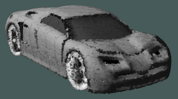
Shading is the biggest problem here, and the shading problem is mainly a lighting problem. Lighting for solid objects means a mix of – diffuse+specular reflection; shadows; and global illumination. Computing diffuse and specular reflection requires a normal, something which particles do not really have, unless we fake it. So that was my first line of attack – generate a normal for the particle. It would need to be consistent with the shape of the system, locally and globally, if it was going to give a good lighting approximation. I tried to use the position of the particle to generate a normal. It turns out that’s rather difficult if you’ve got something other than a load of static particles in the shape of a sphere or box. Then I tried to use a mesh as an emitter and use the underlying normal from the mesh for the particle. It did work, but of course once the particle moves away from it’s spawn point it becomes less and less accurate.
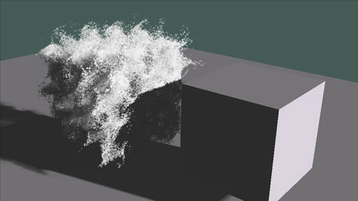
The image here shows particles generated from the car mesh in Frameranger, matching the shading and lighting.
I needed a better reference, so I looked away from solid objects and had a look at how you would light a volumetric object – e.g. a cloud. Which in real life is actually millions of millions of little particles, so maybe it makes quite a good match to lighting, well.. particles. It works out as a model of scattering and absorbtion. You cast light rays into the volume, and ray march through it. Whenever the ray hits a cell that isnt empty, a bit of the light gets absorbed by the cell and a bit of it scattered along secondary rays in different directions, and the rest passes on to the next cell. The cell’s brightness is the amount of light remaining on the ray when it gets to that cell. Scattering properly is hideously slow and expensive so we’ll just completely ignore it, and instead add a global constant to fake it (a good old “ambient” term). That just leaves us with marching rays through the volume and subtracting a small amount per cell, scaled by the amount of stuff in the cell. This actually works great, and I’ve used it for shading realtime smoke simulations – with a few additional constraints, like fixing to directional lights only and from a fixed direction, you can do it pretty efficiently. It looks superb too.
The problem is that the particles are not in a format that is appropriate for ray marching (like a volume texture). But the look is great – we just need a way of achieving it for particles. What we’re dealing with is semi-transparent things casting shadows, so it makes sense to research how to handle that. The efficient way of handling shadows for things nowadays is to use shadow maps. But shadow maps only work for opaque things – they give you the depth of the closest thing at each point in a 2D projection of light space. For alpha things you need more information than that, because otherwise the shadows will be solid.
Or do you? The first thing I tried was very simple – to use exponential shadow maps. Exponential shadowmaps have a great artefact / bug where the shadow seems to fade in close to the caster, and this is usually annoying – but for semi-transparent stuff we can use it to our advantage. Yep, plain old exponential shadowmaps actually work pretty well as shadowmaps for translucent objects – as long as those translucent objects aren’t all that translucent (e.g. smoke volumes). The blur step also makes small casters soften with those around them. It’s pretty fast too, and it almost drops into your regular lighting pipeline. But, for properly transparent (low alpha) stuff like particles, it’s not quite good enough.
The really nice high end offline way is to use deep shadow maps. That basically gives you a function or curve that gives you the shadow intensity at a given depth value. It’s usually generated by buffering up all the values written to each pixel in the map (depth and alpha), sorting them, and fitting a curve to them which is stored. Unfortunately it doesn’t map too well to pixel shader hardware. However there is a discrete version which is much simpler – opacity shadow maps. For this you divide depth into a series of layers and sum up the alpha value sums at each layer for the stuff written with a depth greater than that layer. On modern GPUs that’s actually pretty easy – you can fit 16 layers into 4 MRTs of 4 channels each, and render them in one pass! Unfortunately it’s not expandable beyond that without adding more passes, but it’s good enough to be getting on with – as long as you don’t need to cover a really large depth range and the layers are too spaced out. But this gives us nice shadows which work with semi-transparent stuff properly. You could even do coloured shadows if you didn’t mind less layers or multiple passes.
The next issue is how to apply that shadow information to the particles – it requires samping from 4 maps plus a bunch of maths, and isn’t all that quick. If we did it for every pixel rendered for the particles, it’d hammer the already stressed pixelshader. If the particles are small enough we could just sample it once per particle in the vertex shader – but it’s too many textures to sample. Fortunately the solution is easy – just calculate a colour buffer using the fragment shader, with all the lighting and shading information per particle in it, and sample that in the vertex shader. The great thing about that is it’s really similar in concept to the deferred renderer I’ve already got for solid geometry. You have a buffer containing positions and other information; you perform the lighting in multiple passes, one per light, blending into a composite buffer; then sample that composite buffer to get the particle colour when rendering to the screen. It’s so similar in fact to the deferred rendering pipeline that I can use the almost same lighting code, and even the same shadow maps from solid geometry to apply to the particles too – so particles can cast shadows on geometry, and geometry can cast shadows on particles.
This shading pipeline – compositing first to a buffer, one pixel per particle – opens up new options. We can do all the same tricks we do in deferred rendering, like indexing a lookup table which contains material parameters for example. Or apply environment maps as well as lights. Or perform more complicated operations like using the particle’s life to index a colour lookup texture and change colour over the life of the particle – make it glow at first then fade down. It allows multiple operations to be glued together as separate passes rather than making many combinations of one shader pass.
So, we have a particle colour in a buffer. The next job is to render the particles to the screen. We’ve gone to all this effort to colour them well that we need to consider sorting – back to front – so it actually looks right. This could be problematic – we’ve got 1 million+ particles to sort, all moving independently and potentially quite quickly and randomly, and it has to be done on the GPU not the CPU – we can’t be pulling them back to CPU just to sort.
I had read some papers on sorting on the GPU but I decided it looked totally evil, so I ignored them. My first sorting approach was basically a bucket sort on GPU. I created a series of “buckets” – between 16 and 64 slices the size of the screen, laid out on a 2d texture (which was massive, by the way), with z values from the near to the far plane. Then I rendered the particles to that slice target, and in the vertex shader I worked out which slice fit the particle’s viewspace z value, and offset the output position to be in that slice. So, in one pass I had rendered all the particles to their correct “buckets” – all I had to do was to blend the buckets to the main screen from back to front, and I got a nicely sorted particle render which rendered efficiently – not much slower than not sorting at all. Unfortunately it had some problems – it used an awful lot of VRAM for the slice target, and the granularity of the slices was poor – they were too spread out, so sometimes all the particles would end up in one slice and not be sorted at all. I improved the Z ranges of the slices to fit the approximate (i.e. guessed) bound box of the particle system, but it still didn’t have great precision. In the end on Frameranger the VRAM requirements were simply too high, and I had to drop the effect. It turns out that the layers method is very useful for other things though, like rendering particles into volumes or arbitrary-layered opacity shadow maps.
When I revisted the particle effect, I knew the sorting had to be fixed. I looked back at the papers on GPU sorting, specifically the one in GPU Gems. They seemed very heavyweight – a sort of a 1024×1024 buffer (i.e. 1 million particles) would require 210 passes over that buffer per frame, which is completely unfeasible on a current high end GPU. But there was one line which caught my attention – “This will allow us to use intermediate results of the algorithm that converge to the correct sequence while we do more passes incrementally”. One of the sorting techniques would work over multiple frames – i.e. for each iteration of the algorithm, the results would be more sorted than the previous iteration – it would not give randomly changing orders, but converge on a sorted order. Perfect – we could split the sort over N frames, and it would get better and better each frame. That’s exactly what I did, and it actually worked great. It used much less memory than the bucket sort method and gave better accuracy too – and the performance requirements could be scaled as necessary in exchange for more frames needed to sort.
There are some irritations with simulating particles on GPU. Each particle must be treated independently and you have to perform a whole pass on all the particles simultaneously. It makes things which are trivial on CPU, like counting how many particles you emitted so far that frame, very difficult or not feasible at all on GPU. But it’s a rather important thing to solve – you often need to be able to emit particles slowly over time, rather than all at once. The first way I tried to solve that was to use the location of the particle in the position buffer. I would for example emit the particles in the y range 0 to 0.1 on the first frame, than 0.1 to 0.2 on the next, and so on. It worked to a point, but fell down when I started randomising the particle’s lifetime – I needed to emit different particles at different times. Then I realised something useful. If you’re dealing with loads and loads of something – like a near infinite amount – then doing things randomly is as good as doing things correctly. I.e. I dont need to correctly emit say 100 particles this frame – I just need to try to emit e.g. roughly 1% of particles this frame and if I’ve got enough particles in the first place, it’ll look alright. The trick is that those 1% is the right amount of random.
I’ll explain. The update goes like this: 1. generate a buffer of new potential spawn positions for particles. 2. Update the particle position buffer by reading the old positions, applying the particle velocities to them, and reducing the life; then if the life is less than 0, pick the corresponding value from the spawn position buffer and write that out instead. So, each frame I generate a whole set of spawn positions for the particles, but they only get used if the particle dies. But how to control the emission? Clearly if I put a value in the spawn buffer which has an initial life of less than 0 and it gets used, it’ll get killed by the renderer anyway and the next frame around it’ll respawn again – i.e. the particle never gets rendered and doesn’t really get spawned either. So if I want to control the number of particles emitted I just limit the number of values in the spawn buffer each frame that have an initial life greater than 0.
How do I choose which spawn values have valid lives? It needs to be a good spread, because the emission life is also randomised – some particles die earlier than others and need respawning. If I simply use a rolling window it’s not random enough and particles stop being spawned properly. If I actually randomly choose, it’s too random – it becomes dependent on framerate, and on a fast machine the particles just all get spawned – the randomness makes it run through the buffer too fast. So, what I did was a compromise between them – a random value that slowly changes in a time-dependent way.
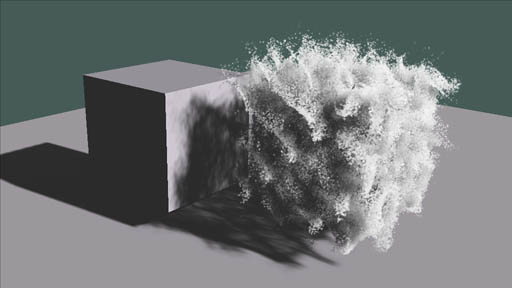
The other nice thing about this spawn buffer was that it made it easy to combine multiple emitters. I could render some of the spawn buffer from one emitter, some from other, and it would “just work”. One of the first emitters I tried was a mesh emitter. The obvious way would be to emit particles from the vertices but this only worked well for some meshes – so instead I generated a texture of random positions on the mesh surface. I did this by firstly determining the total area of all the triangles in the mesh; then for each triangle spawning a number of particles, which was the total number of particles * (triangle area / total area). To spawn random positions I just used a random barycentric coordinate.
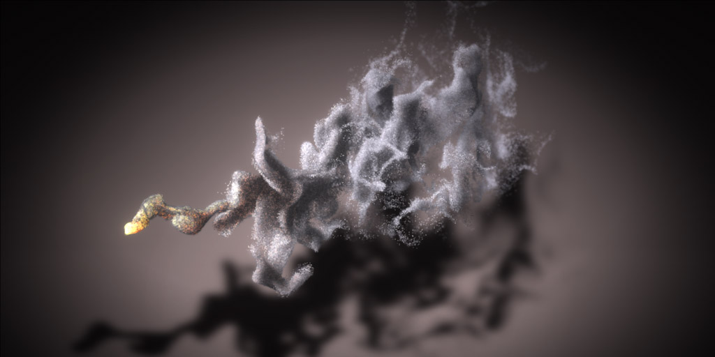
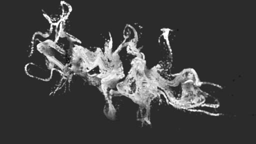
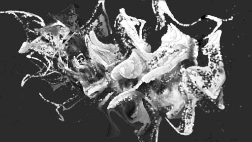
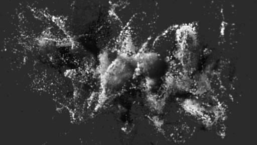
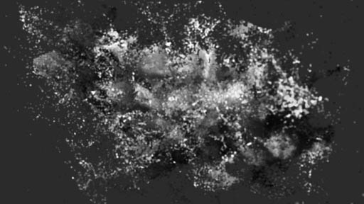
Here’s an early test case with particles generated for a logo mesh and being affected by fluid.
Finally I needed some affectors. Of course I did the usual forces, but I wanted fluid dynamics. The obvious idea was to use a 3d grid solver and drive the particles by the velocities. Well, that wasn’t great. The main problem was that the grid was limited to a small area, and the particles could go anywhere. Besides, the fluid solver was quite slow to update for a decent resolution. So I used a much simpler method that generated much better results – procedural fluid flows (thanks Mr Bridson). Essentially this fakes up a velocity field by using differentials of a perlin-style noise field to generate fluid-like eddies – “curl noise”. By layering several of these on top, combined with some simple velocities, it looked very much like fluid.
The one remaining affector was something to attract particles to images. To do this I generated a texture from the image where each pixel contained the position of the closest filled pixel in the source image – a bit like a distance field but storing the closest position rather than the distance. Then, in the shader I projected the particle into image space, looked up the closest pixel and used that to calculate a velocity, weighted by the distance from the pixel. With a bit of randomness and adjustment to stop it affecting very new or very old particles, it worked a charm.

And there we have it – a “modern” particle system that works on DirectX9 – no CUDA required! I’m sure this will develop over time. With better GPUs the particle counts will go up fast – between 4 and 16 million is workable already on a top end Geforce, and it’ll go up and up with future hardware generations. In fact I have a host of other renderers for the particles besides this simple one – things to do metaballs, volume renders and clouds, for example – and a load of other improvements, but that can wait for another demo..
By the way, there’s a nice thing about GPU particles that maybe isn’t immediately obvious. You’re writing all the behaviour code (emission, affectors..) in shaders, right? And you can probably reload your shaders on the fly in your working environment. All of a sudden it makes development a lot easier. You don’t need to recompile and reload the executable every time you change the code, you can simply edit and reload the shader in the live environment. Great eh?